Week - 11 Demand Forecasting [Store Sales Prediction]
Nowadays, shopping malls and Big Marts keep track of individual items sales data in order to forecast future client demand and adjust inventory management. In a data warehouse, these data stores hold a significant amount of consumer information and particular item details. By mining the data store from the data warehouse, more anomalies and patterns can be discovered.
Store Sales Prediction as a Demand Forecasting Usecase?
Store sales prediction is a demand forecasting usecase in manufacturing indust. By analyzing store sales data, manufacturers can gain insights into customer demand patterns, which can help to inform production and inventory decisions. For example, a manufacturer may analyze store sales data to determine which products are selling well and which products are not, and then adjust production schedules and inventory levels accordingly. This can help the manufacturer to better manage stock levels, reduce waste, and ensure that popular products are always in stock. By using store sales data as part of a demand forecasting process, manufacturers can make more informed decisions that ultimately lead to improved business performance.
AI Project Cycle 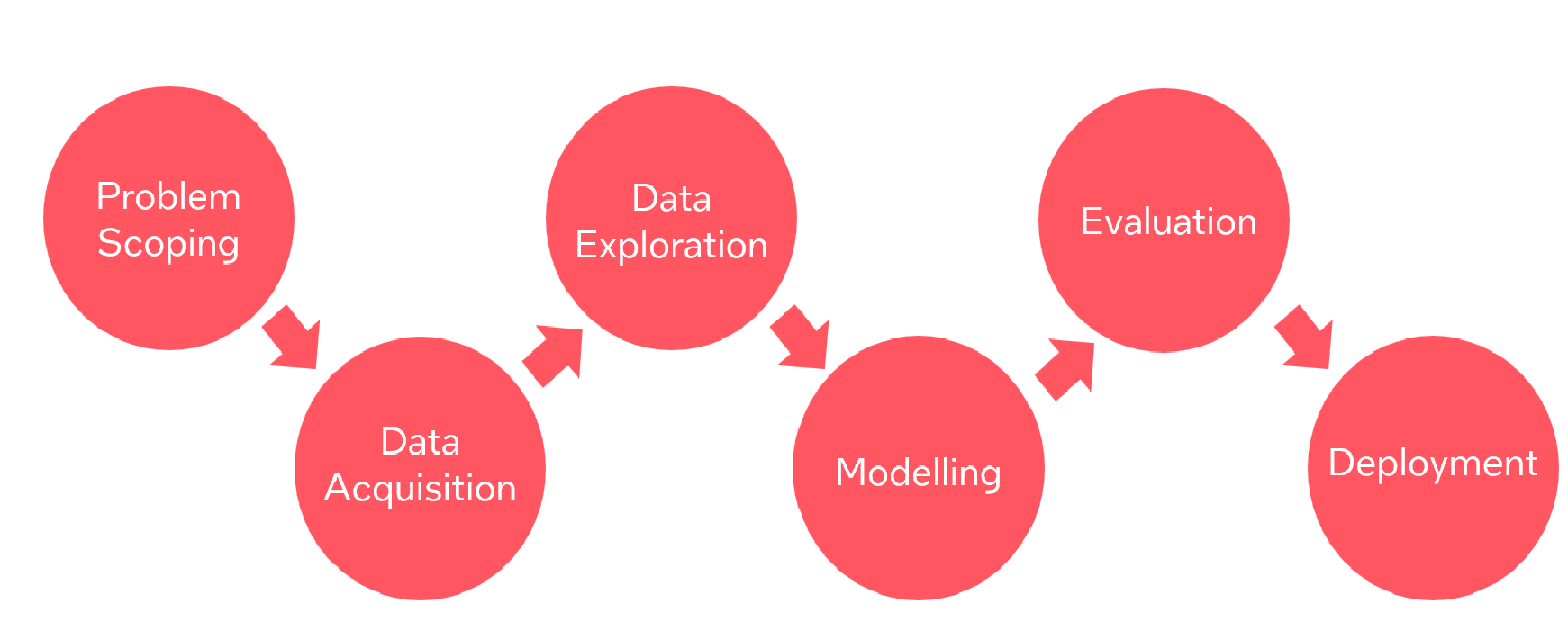 

Context: Understanding the Problem Statement --------Problem Scoping (AI Project Cycle - Step 1)
Nowadays, shopping malls and Big Marts keep track of individual items sales data in order to forecast future client demand and adjust inventory management. In a data warehouse, these data stores hold a significant amount of consumer information and particular item details. By mining the data store from the data warehouse, more anomalies and patterns can be discovered.
The classical machine learning tasks like Data Exploration, Data Cleaning, Feature Engineering, Model Building and Model Testing. Try out different machine learning algorithms that’s best fit for the above case.
Import the useful Packages & Libraries
%pip install ipython-autotime
%load_ext autotime
Requirement already satisfied: ipython-autotime in c:\Program Files\Python314\Lib\site-packages (0.3.2)
Requirement already satisfied: ipython in C:\Users\joann\AppData\Roaming\Python\Python314\site-packages (from ipython-autotime) (9.17.1)
Requirement already satisfied: colorama>=0.4.4 in C:\Users\joann\AppData\Roaming\Python\Python314\site-packages (from ipython->ipython-autotime) (0.4.6)
Requirement already satisfied: ipython-pygments-lexers>=1.0.0 in C:\Users\joann\AppData\Roaming\Python\Python314\site-packages (from ipython->ipython-autotime) (1.1.1)
Requirement already satisfied: jedi>=0.18.2 in C:\Users\joann\AppData\Roaming\Python\Python314\site-packages (from ipython->ipython-autotime) (0.20.0)
Requirement already satisfied: matplotlib-inline>=0.1.6 in C:\Users\joann\AppData\Roaming\Python\Python314\site-packages (from ipython->ipython-autotime) (0.2.2)
Requirement already satisfied: prompt_toolkit<3.1.0,>=3.0.41 in C:\Users\joann\AppData\Roaming\Python\Python314\site-packages (from ipython->ipython-autotime) (3.0.53)
Requirement already satisfied: psutil>=7 in C:\Users\joann\AppData\Roaming\Python\Python314\site-packages (from ipython->ipython-autotime) (7.2.2)
Requirement already satisfied: pygments>=2.14.0 in C:\Users\joann\AppData\Roaming\Python\Python314\site-packages (from ipython->ipython-autotime) (2.21.0)
Requirement already satisfied: stack_data>=0.6.0 in C:\Users\joann\AppData\Roaming\Python\Python314\site-packages (from ipython->ipython-autotime) (0.6.3)
Requirement already satisfied: traitlets>=5.13.0 in C:\Users\joann\AppData\Roaming\Python\Python314\site-packages (from ipython->ipython-autotime) (5.16.1)
Requirement already satisfied: wcwidth>=0.1.4 in C:\Users\joann\AppData\Roaming\Python\Python314\site-packages (from prompt_toolkit<3.1.0,>=3.0.41->ipython->ipython-autotime) (0.9.2)
Requirement already satisfied: parso<0.9.0,>=0.8.6 in C:\Users\joann\AppData\Roaming\Python\Python314\site-packages (from jedi>=0.18.2->ipython->ipython-autotime) (0.8.7)
Requirement already satisfied: executing>=1.2.0 in C:\Users\joann\AppData\Roaming\Python\Python314\site-packages (from stack_data>=0.6.0->ipython->ipython-autotime) (2.2.1)
Requirement already satisfied: asttokens>=2.1.0 in C:\Users\joann\AppData\Roaming\Python\Python314\site-packages (from stack_data>=0.6.0->ipython->ipython-autotime) (3.0.2)
Requirement already satisfied: pure-eval in C:\Users\joann\AppData\Roaming\Python\Python314\site-packages (from stack_data>=0.6.0->ipython->ipython-autotime) (0.2.4)
Note: you may need to restart the kernel to use updated packages.
time: 98.7 μs (started: 2026-10-06 16:58:25 -07:00)
# if not already, install matplotlib seaborn plotlytime: 1.02 ms (started: 2026-10-06 16:58:25 -07:00)
import numpy as np
import pandas as pd
import matplotlib.pyplot as plt
import seaborn as sns
import plotly.express as px
import warnings
warnings.filterwarnings(action="ignore")
#plt.style.use(["seaborn-bright","dark_background"])
time: 2.39 s (started: 2026-10-06 16:58:25 -07:00)
To know more about Plotly click here
Dataset: Data Acquisition (AI Project Cycle - Step 2)
Data is taken from kaggle which is a Store Sales Dataset.
Source - https://
Load/Read the Dataset
# Load the data
train = pd.read_csv("Data11/Train.csv")
test = pd.read_csv("Data11/Test.csv")
time: 42.6 ms (started: 2026-10-06 16:58:27 -07:00)
View the data
#Prints the first five entry of the dataframe
train.head()time: 27 ms (started: 2026-10-06 16:58:27 -07:00)
test.head()time: 16.9 ms (started: 2026-10-06 16:58:27 -07:00)
#It shows the number of rows and columns of the given dataframe
train.shape
(8523, 12)time: 3.02 ms (started: 2026-10-06 16:58:27 -07:00)
#It shows the number of rows and columns of the given dataframe
test.shape
(5681, 11)time: 3.29 ms (started: 2026-10-06 16:58:27 -07:00)
- We have train(8523) and test(5681) data set, train data set has both input and output variables.
Attribute Information-
Features:
Item_weight : Weight of product
Item_Fat_Content : Whether the product is low fat or not
Item_Visibility : The % of total display area of all products in a store allocated to a particular product.
Item_Type : The category to which the product belongs
Item_MRP : Maximum Retail Price (list price) of the product
Outlet_Identifier : Unique Store ID
Outlet_Establishment_Year : The year in which store was established
Outlet_Size : The size of the store in terms of ground area covered
Outlet_Location_Type : The type of city in which the store is located
Outlet_Type : Whether the outlet is just a grocery store or some sort of supermarket
Target:
Item_Outlet_Sales : Sales of the product in the particular store. This is the outcome variable to be predicted.
Data Preprocessing ------ Data Exploration(AI Project Cycle - Step 3)
View the information of data
# info() helps summarize the dataset- It gives basic information like number of non-null values, datatypes and memory usage
# It is a good practise to start by this information
train.info()
<class 'pandas.DataFrame'>
RangeIndex: 8523 entries, 0 to 8522
Data columns (total 12 columns):
# Column Non-Null Count Dtype
--- ------ -------------- -----
0 Item_Identifier 8523 non-null str
1 Item_Weight 7060 non-null float64
2 Item_Fat_Content 8523 non-null str
3 Item_Visibility 8523 non-null float64
4 Item_Type 8523 non-null str
5 Item_MRP 8523 non-null float64
6 Outlet_Identifier 8523 non-null str
7 Outlet_Establishment_Year 8523 non-null int64
8 Outlet_Size 6113 non-null str
9 Outlet_Location_Type 8523 non-null str
10 Outlet_Type 8523 non-null str
11 Item_Outlet_Sales 8523 non-null float64
dtypes: float64(4), int64(1), str(7)
memory usage: 799.2 KB
time: 17 ms (started: 2026-10-06 16:58:27 -07:00)
# info() helps summarize the dataset- It gives basic information like number of non-null values, datatypes and memory usage
# It is a good practise to start by this information

# Write code to illustrate the information about test dataset
time: 1.4 ms (started: 2026-10-06 16:58:27 -07:00)
Check the number of rows and columns of the dataset
#It returns the column names of the given dataframe
train.columns
Index(['Item_Identifier', 'Item_Weight', 'Item_Fat_Content', 'Item_Visibility',
'Item_Type', 'Item_MRP', 'Outlet_Identifier',
'Outlet_Establishment_Year', 'Outlet_Size', 'Outlet_Location_Type',
'Outlet_Type', 'Item_Outlet_Sales'],
dtype='str')time: 3.48 ms (started: 2026-10-06 16:58:27 -07:00)
#It returns the column names of the given dataframe
test.columns
Index(['Item_Identifier', 'Item_Weight', 'Item_Fat_Content', 'Item_Visibility',
'Item_Type', 'Item_MRP', 'Outlet_Identifier',
'Outlet_Establishment_Year', 'Outlet_Size', 'Outlet_Location_Type',
'Outlet_Type'],
dtype='str')time: 4.4 ms (started: 2026-10-06 16:58:27 -07:00)
#It gives the numerical statistical information of the dataframe
"""
count - The number of non-empty values.
mean - The average value
std - The standard deviation
min - the minimum value
25% - The 25% percentile*
50% - The 50% percentile*
75% - The 75% percentile*
max - the maximum value """

train.describe()time: 33.1 ms (started: 2026-10-06 16:58:27 -07:00)
test.describe()time: 28.4 ms (started: 2026-10-06 16:58:27 -07:00)
Find the total number of missing values feature wise
#It returns the number of null values in the dataframe for every column feature
#Using info() we can view the number of non-null values whereas isnull() gives the number of null values
train.isnull().sum()time: 17 ms (started: 2026-10-06 16:58:27 -07:00)
We have 17% and 28% of missing values in Item weight and Outlet_Size columns respectively.
Why missing values treatment is required?
Missing data in the training data set can reduce the power / fit of a model or can lead to a biased model because we have not analysed the behavior and relationship with other variables correctly. It can lead to wrong prediction.
#Checking if there is any gender imbalance in dataframe
train['Outlet_Size'].value_counts() time: 11.7 ms (started: 2026-10-06 16:58:27 -07:00)
Since the outlet_size is a categorical column, we can impute the missing values by “Mode”(Most Repeated Value) from the column.
train["Outlet_Size"] = train["Outlet_Size"].fillna(train["Outlet_Size"].mode())time: 5.4 ms (started: 2026-10-06 16:58:27 -07:00)
group = train.groupby("Item_Type")["Item_Weight"].mean()
grouptime: 14 ms (started: 2026-10-06 16:58:27 -07:00)
for i in range(len(group)):
    g = (train['Item_Type'] == group.index[i]) & (train['Item_Weight'].isna() == True)
    train['Item_Weight'] = np.select([g], [group.iloc[i]], train['Item_Weight'])
time: 45.2 ms (started: 2026-10-06 16:58:27 -07:00)
train.describe()time: 42.2 ms (started: 2026-10-06 16:58:28 -07:00)
fig = px.box(train, x = "Item_Outlet_Sales",height=400,width=700)
#fig.show()
fig.show(renderer="browser")
time: 742 ms (started: 2026-10-06 16:58:28 -07:00)
q1 = train["Item_Outlet_Sales"].quantile(0.25)
q3 = train["Item_Outlet_Sales"].quantile(0.75)
iqr = q3 - q1
upper_bound = q3+1.5*iqr
time: 12.9 ms (started: 2026-10-06 16:58:28 -07:00)
group1 = train.groupby("Item_Type")["Item_Outlet_Sales"].mean()
group1time: 40.2 ms (started: 2026-10-06 16:58:28 -07:00)
for i in range(len(group1)):
    g = (train['Item_Type'] == group1.index[i]) & (train['Item_Outlet_Sales'] > upper_bound)
    train['Item_Outlet_Sales'] = np.select([g], [group1.iloc[i]], train['Item_Outlet_Sales'])
time: 54.8 ms (started: 2026-10-06 16:58:29 -07:00)
for i in train.columns:
    if train[i].dtype=="object":
        print("{} has unique values {}".format(i,train[i].unique()))
time: 2.25 ms (started: 2026-10-06 16:58:29 -07:00)
Every dataset consists of some missing values and outliers. The categorical missing values are filled with most frequent value i.e. mode while the numeric values are filled with mean. Also the outliers are treated with the mean value correspoiding to their item type.
Feature Encoding
We use one-hot encoding to convert categorical features to numeric data. For more info on one hot encoding clic here
Since the outlet_size is a categorical column, we can impute the missing values by “Mode”(Most Repeated Value) from the column.
train["Item_Fat_Content"] = train["Item_Fat_Content"].replace(['Low Fat','Regular','low fat','LF','reg'],
                                                              ['Low Fat','Regular','Low Fat','Low Fat','Regular'])
time: 14.9 ms (started: 2026-10-06 16:58:29 -07:00)
train["Item_Type"] = train["Item_Type"].replace(['Dairy','Soft Drinks','Meat','Fruits and Vegetables',
                                                 'Household','Baking Goods','Snack Foods','Frozen Foods',
                                                 'Breakfast','Health and Hygiene','Hard Drinks','Canned',
                                                 'Breads','Starchy Foods','Others','Seafood'],
                                               ['Food','Drinks','Food','Food',
                                                 'Others','Others','Food','Food',
                                                 'Food','Others','Drinks','Food',
                                                 'Food','Food','Others','Food'])
time: 28.5 ms (started: 2026-10-06 16:58:29 -07:00)
train["Outlet_Location_Type"] = train["Outlet_Location_Type"].replace(['Tier 1','Tier 3','Tier 2'],
                                                                      [1,3,2])
time: 14.6 ms (started: 2026-10-06 16:58:29 -07:00)
Data Visualizations
plt.figure(figsize=(5,3))
sns.countplot(x = "Item_Fat_Content", data = train)
plt.title("Item Fat Content")
plt.show()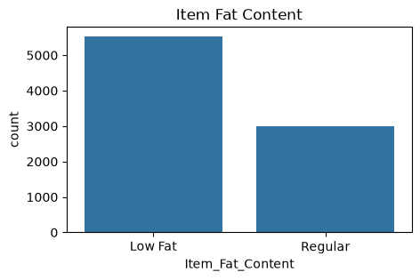
time: 214 ms (started: 2026-10-06 16:58:29 -07:00)
plt.figure(figsize=(14,5))
sns.countplot(x = "Item_Type", data = train)
plt.title("Item Type")
plt.xticks(rotation=45)
plt.show()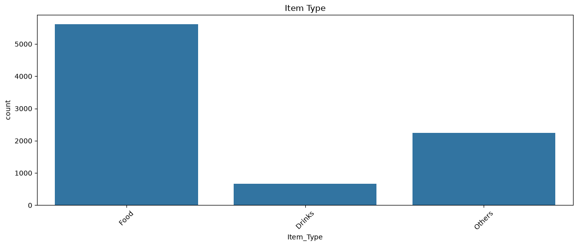
time: 193 ms (started: 2026-10-06 16:58:29 -07:00)
plt.figure(figsize=(6,3))
sns.countplot(x = "Outlet_Size", data = train)
plt.title("Outlet Size")
plt.show()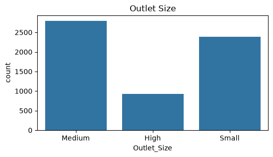
time: 180 ms (started: 2026-10-06 16:58:29 -07:00)
train["sqr_Item_Outlet_Sales"] = np.sqrt(train["Item_Outlet_Sales"])time: 5.85 ms (started: 2026-10-06 16:58:29 -07:00)
train.columns,train.shape(Index(['Item_Identifier', 'Item_Weight', 'Item_Fat_Content', 'Item_Visibility',
'Item_Type', 'Item_MRP', 'Outlet_Identifier',
'Outlet_Establishment_Year', 'Outlet_Size', 'Outlet_Location_Type',
'Outlet_Type', 'Item_Outlet_Sales', 'sqr_Item_Outlet_Sales'],
dtype='str'),
(8523, 13))time: 6.21 ms (started: 2026-10-06 16:58:29 -07:00)
Correlation Heatmap
To know more about heatmap click here
sns.heatmap(train.corr(numeric_only=True),annot=True)
plt.show()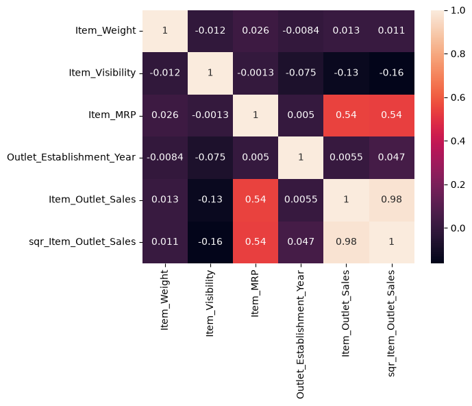
time: 477 ms (started: 2026-10-06 16:58:30 -07:00)
A correlation coefficient of 0.5 indicates a moderate positive linear relationship between two variables. This means that as one variable increases, the other variable tends to increase as well.
train["cbr_Item_Visibility"] = np.cbrt(train["Item_Visibility"])time: 2.96 ms (started: 2026-10-06 16:58:30 -07:00)
One-Hot Encoding
category_col = ['Item_Fat_Content','Item_Type','Outlet_Size','Outlet_Type']time: 1.43 ms (started: 2026-10-06 16:58:30 -07:00)
train = pd.get_dummies(train,columns=category_col,drop_first=False)time: 19.8 ms (started: 2026-10-06 16:58:30 -07:00)
train.drop(columns=["Item_Identifier","Outlet_Identifier","Outlet_Establishment_Year","sqr_Item_Outlet_Sales","Item_Visibility"],inplace=True)time: 3.02 ms (started: 2026-10-06 16:58:30 -07:00)
train.to_csv("Data11/modified_train.csv",index=False)time: 187 ms (started: 2026-10-06 16:58:30 -07:00)
# Write code to print training dataframetime: 984 μs (started: 2026-10-06 16:58:30 -07:00)
Working on test data same as we work on train data
for i in test.columns:
    per = test[i].isnull().sum()/len(test)
    print("Feature {} has {}% data missing".format(i,round(per*100,3)))
Feature Item_Identifier has 0.0% data missing
Feature Item_Weight has 17.18% data missing
Feature Item_Fat_Content has 0.0% data missing
Feature Item_Visibility has 0.0% data missing
Feature Item_Type has 0.0% data missing
Feature Item_MRP has 0.0% data missing
Feature Outlet_Identifier has 0.0% data missing
Feature Outlet_Establishment_Year has 0.0% data missing
Feature Outlet_Size has 28.27% data missing
Feature Outlet_Location_Type has 0.0% data missing
Feature Outlet_Type has 0.0% data missing
time: 11.2 ms (started: 2026-10-06 16:58:30 -07:00)
test["Outlet_Size"] = test["Outlet_Size"].fillna(test["Outlet_Size"].mode())time: 6.73 ms (started: 2026-10-06 16:58:30 -07:00)
for i in range(len(group)):
    g = (test['Item_Type'] == group.index[i]) & (test['Item_Weight'].isna() == True)
    test['Item_Weight'] = np.select([g], [group.iloc[i]], test['Item_Weight'])
time: 70.5 ms (started: 2026-10-06 16:58:30 -07:00)
test["Item_Fat_Content"] = test["Item_Fat_Content"].replace(['Low Fat','Regular','low fat','LF','reg'],
                                                              ['Low Fat','Regular','Low Fat','Low Fat','Regular'])
time: 12.3 ms (started: 2026-10-06 16:58:31 -07:00)
test["Item_Type"] = test["Item_Type"].replace(['Dairy','Soft Drinks','Meat','Fruits and Vegetables',
                                                 'Household','Baking Goods','Snack Foods','Frozen Foods',
                                                 'Breakfast','Health and Hygiene','Hard Drinks','Canned',
                                                 'Breads','Starchy Foods','Others','Seafood'],
                                               ['Food','Drinks','Food','Food',
                                                 'Others','Others','Food','Food',
                                                 'Food','Others','Drinks','Food',
                                                 'Food','Food','Others','Food'])
time: 26.8 ms (started: 2026-10-06 16:58:31 -07:00)
test["Outlet_Location_Type"] = test["Outlet_Location_Type"].replace(['Tier 1','Tier 3','Tier 2'],
                                                                      [1,3,2])
time: 6.07 ms (started: 2026-10-06 16:58:31 -07:00)
test["cbr_Item_Visibility"] = np.cbrt(test["Item_Visibility"])time: 2.74 ms (started: 2026-10-06 16:58:31 -07:00)
test = pd.get_dummies(test,columns=category_col,drop_first=False)time: 16.8 ms (started: 2026-10-06 16:58:31 -07:00)
test.drop(columns=["Item_Identifier","Outlet_Identifier","Outlet_Establishment_Year","Item_Visibility"],inplace=True)time: 2.75 ms (started: 2026-10-06 16:58:31 -07:00)
X = train.drop(columns=["Item_Outlet_Sales"])time: 7.23 ms (started: 2026-10-06 16:58:31 -07:00)
test = test[X.columns]time: 6.38 ms (started: 2026-10-06 16:58:31 -07:00)
test.to_csv("Data11/modified_test.csv",index=False)time: 60.3 ms (started: 2026-10-06 16:58:31 -07:00)
test.head()time: 23.3 ms (started: 2026-10-06 16:58:31 -07:00)
Splitting the dataframe into independent(features) and dependent features(targets)
train = pd.read_csv("Data11/modified_train.csv")
test = pd.read_csv("Data11/modified_test.csv")
time: 82.5 ms (started: 2026-10-06 16:58:31 -07:00)
X = train.drop(columns=["Item_Outlet_Sales"])
y = train["Item_Outlet_Sales"]
time: 3.61 ms (started: 2026-10-06 16:58:31 -07:00)
from sklearn.model_selection import train_test_split
x_train, x_valid, y_train, y_valid = train_test_split(X,y,test_size=0.2,random_state=101)
time: 433 ms (started: 2026-10-06 16:58:31 -07:00)
Building a Model ------ Modeling ( AI Project Cycle - Step 4)
To learn more about the sklearn evaluation matrices click here
from sklearn.metrics import mean_squared_error,mean_absolute_error,r2_score
import time
time: 1.56 ms (started: 2026-10-06 16:58:32 -07:00)
from sklearn.linear_model import LinearRegression,Lasso,Ridge
from sklearn.tree import DecisionTreeRegressor
from sklearn.ensemble import RandomForestRegressor,ExtraTreesRegressor,AdaBoostRegressor,GradientBoostingRegressor
from sklearn.svm import SVR
from sklearn.neighbors import KNeighborsRegressor
time: 234 ms (started: 2026-10-06 16:58:32 -07:00)
models = []
models.append(("LinearRegressor",LinearRegression()))
models.append(("Lasso",Lasso()))
models.append(("Ridge",Ridge()))
models.append(("DecisionTree",DecisionTreeRegressor()))
models.append(("RandomForestRegressor",RandomForestRegressor()))
models.append(("ExtraTreeRegressor",ExtraTreesRegressor()))
models.append(("AdaBoostRegressor",AdaBoostRegressor()))
models.append(("GradientBoosingRegressor",GradientBoostingRegressor()))
models.append(("SVR",SVR()))
models.append(("KNeighborsRegressor",KNeighborsRegressor()))
time: 3.76 ms (started: 2026-10-06 16:58:32 -07:00)
Evaluating the Model ------- Evaluation (AI Project Cycle - Step 5)
names = []
score = []
rmse = []
mse = []
mae = []
r2 = []
timing = []
time: 125 ms (started: 2026-10-06 16:58:32 -07:00)
for name,model in models:
    model = model
    beg = time.time()
    model.fit(x_train,y_train)
    pred = model.predict(x_valid)
    end = time.time()
    print("Model = {}".format(name))
    print("Score = {}, RMSE = {}, MSE = {}, MAE = {}, R2 = {},Time = {}\n".format(round(model.score(x_valid,y_valid),4),
                                                round(np.sqrt(mean_squared_error(pred,y_valid)),4),
                                                round(mean_squared_error(pred,y_valid),4),
                                                round(mean_absolute_error(pred,y_valid),4),
                                                round(r2_score(y_valid,pred),4),(end-beg)))
    names.append(name)
    score.append(round(model.score(x_valid,y_valid),4))
    rmse.append(round(np.sqrt(mean_squared_error(pred,y_valid)),4))
    mse.append(round(mean_squared_error(pred,y_valid),4))
    mae.append(round(mean_absolute_error(pred,y_valid),4))
    r2.append(round(r2_score(pred,y_valid),4))
    timing.append(end-beg)
Model = LinearRegressor
Score = 0.5206, RMSE = 1029.5462, MSE = 1059965.435, MAE = 791.8425, R2 = 0.5206,Time = 0.011135101318359375
Model = Lasso
Score = 0.5207, RMSE = 1029.4332, MSE = 1059732.8016, MAE = 791.6892, R2 = 0.5207,Time = 0.006826162338256836
Model = Ridge
Score = 0.5206, RMSE = 1029.5423, MSE = 1059957.2803, MAE = 791.845, R2 = 0.5206,Time = 0.0054781436920166016
Model = DecisionTree
Score = 0.0514, RMSE = 1448.2749, MSE = 2097500.1175, MAE = 1031.009, R2 = 0.0514,Time = 0.0448911190032959
Model = RandomForestRegressor
Score = 0.486, RMSE = 1066.147, MSE = 1136669.3879, MAE = 766.3479, R2 = 0.486,Time = 2.812385320663452
Model = ExtraTreeRegressor
Score = 0.4487, RMSE = 1104.1443, MSE = 1219134.5303, MAE = 795.0229, R2 = 0.4487,Time = 2.0628879070281982
Model = AdaBoostRegressor
Score = 0.5197, RMSE = 1030.6043, MSE = 1062145.2929, MAE = 777.8057, R2 = 0.5197,Time = 0.20270180702209473
Model = GradientBoosingRegressor
Score = 0.5548, RMSE = 992.1315, MSE = 984324.8219, MAE = 719.5038, R2 = 0.5548,Time = 0.8380098342895508
Model = SVR
Score = 0.1931, RMSE = 1335.7496, MSE = 1784227.0399, MAE = 1025.9525, R2 = 0.1931,Time = 3.443126916885376
Model = KNeighborsRegressor
Score = 0.3502, RMSE = 1198.6533, MSE = 1436769.7569, MAE = 893.1281, R2 = 0.3502,Time = 0.08922076225280762
time: 11.9 s (started: 2026-10-06 16:58:32 -07:00)
df = pd.DataFrame()
df["names"] = names
df["Score"] = score
df["time"] = timing
df["rmse"] = rmse
df["mse"] = mse
df["mae"] = mae
df["r2"] = r2
time: 6.46 ms (started: 2026-10-06 16:58:44 -07:00)
df = df.sort_values(by="Score",ascending=False)
fig = px.bar(df,"names","Score",color="names",title="Accuracy Score")
#fig.show()
fig.show(renderer="browser")
time: 443 ms (started: 2026-10-06 16:58:44 -07:00)
# Write code to plot the RMSE values of each model here.time: 2.64 ms (started: 2026-10-06 16:58:45 -07:00)
# Write code to plot the MSE values of each model here.time: 37.3 ms (started: 2026-10-06 16:58:45 -07:00)
# Write code to plot the MAE values of each model here.time: 85.1 ms (started: 2026-10-06 16:58:45 -07:00)
# Write code to plot the R2 Score values of each model here.time: 641 ms (started: 2026-10-06 16:58:45 -07:00)
df = df.sort_values(by="time",ascending=True)
fig = px.bar(df,"names","time",color="names",title="Time taken by each model")
#fig.show()
fig.show(renderer="browser")
time: 1.01 s (started: 2026-10-06 16:58:45 -07:00)
Hyperparameter tuning
for more info on hyperparameter tuning click here
from sklearn import model_selection
classifer = GradientBoostingRegressor()
dt_grid = {'loss':['ls', 'lad', 'huber'],
           'learning_rate':[0.01,0.05,0.1,0.5],
          'n_estimators' : [100,200],
          'max_depth':[3,5,8,10]}
grid_classifier = model_selection.GridSearchCV(classifer, dt_grid, cv=10, refit=True,
                                               return_train_score=True)
grid_classifier.fit(X, y)
results = grid_classifier.cv_results_
print(results.get('params'))
print(results.get('mean_test_score'))
print(results.get('mean_train_score'))
print(grid_classifier.best_params_)
print(grid_classifier.best_score_)
final_model = grid_classifier.best_estimator_
[{'learning_rate': 0.01, 'loss': 'ls', 'max_depth': 3, 'n_estimators': 100}, {'learning_rate': 0.01, 'loss': 'ls', 'max_depth': 3, 'n_estimators': 200}, {'learning_rate': 0.01, 'loss': 'ls', 'max_depth': 5, 'n_estimators': 100}, {'learning_rate': 0.01, 'loss': 'ls', 'max_depth': 5, 'n_estimators': 200}, {'learning_rate': 0.01, 'loss': 'ls', 'max_depth': 8, 'n_estimators': 100}, {'learning_rate': 0.01, 'loss': 'ls', 'max_depth': 8, 'n_estimators': 200}, {'learning_rate': 0.01, 'loss': 'ls', 'max_depth': 10, 'n_estimators': 100}, {'learning_rate': 0.01, 'loss': 'ls', 'max_depth': 10, 'n_estimators': 200}, {'learning_rate': 0.01, 'loss': 'lad', 'max_depth': 3, 'n_estimators': 100}, {'learning_rate': 0.01, 'loss': 'lad', 'max_depth': 3, 'n_estimators': 200}, {'learning_rate': 0.01, 'loss': 'lad', 'max_depth': 5, 'n_estimators': 100}, {'learning_rate': 0.01, 'loss': 'lad', 'max_depth': 5, 'n_estimators': 200}, {'learning_rate': 0.01, 'loss': 'lad', 'max_depth': 8, 'n_estimators': 100}, {'learning_rate': 0.01, 'loss': 'lad', 'max_depth': 8, 'n_estimators': 200}, {'learning_rate': 0.01, 'loss': 'lad', 'max_depth': 10, 'n_estimators': 100}, {'learning_rate': 0.01, 'loss': 'lad', 'max_depth': 10, 'n_estimators': 200}, {'learning_rate': 0.01, 'loss': 'huber', 'max_depth': 3, 'n_estimators': 100}, {'learning_rate': 0.01, 'loss': 'huber', 'max_depth': 3, 'n_estimators': 200}, {'learning_rate': 0.01, 'loss': 'huber', 'max_depth': 5, 'n_estimators': 100}, {'learning_rate': 0.01, 'loss': 'huber', 'max_depth': 5, 'n_estimators': 200}, {'learning_rate': 0.01, 'loss': 'huber', 'max_depth': 8, 'n_estimators': 100}, {'learning_rate': 0.01, 'loss': 'huber', 'max_depth': 8, 'n_estimators': 200}, {'learning_rate': 0.01, 'loss': 'huber', 'max_depth': 10, 'n_estimators': 100}, {'learning_rate': 0.01, 'loss': 'huber', 'max_depth': 10, 'n_estimators': 200}, {'learning_rate': 0.05, 'loss': 'ls', 'max_depth': 3, 'n_estimators': 100}, {'learning_rate': 0.05, 'loss': 'ls', 'max_depth': 3, 'n_estimators': 200}, {'learning_rate': 0.05, 'loss': 'ls', 'max_depth': 5, 'n_estimators': 100}, {'learning_rate': 0.05, 'loss': 'ls', 'max_depth': 5, 'n_estimators': 200}, {'learning_rate': 0.05, 'loss': 'ls', 'max_depth': 8, 'n_estimators': 100}, {'learning_rate': 0.05, 'loss': 'ls', 'max_depth': 8, 'n_estimators': 200}, {'learning_rate': 0.05, 'loss': 'ls', 'max_depth': 10, 'n_estimators': 100}, {'learning_rate': 0.05, 'loss': 'ls', 'max_depth': 10, 'n_estimators': 200}, {'learning_rate': 0.05, 'loss': 'lad', 'max_depth': 3, 'n_estimators': 100}, {'learning_rate': 0.05, 'loss': 'lad', 'max_depth': 3, 'n_estimators': 200}, {'learning_rate': 0.05, 'loss': 'lad', 'max_depth': 5, 'n_estimators': 100}, {'learning_rate': 0.05, 'loss': 'lad', 'max_depth': 5, 'n_estimators': 200}, {'learning_rate': 0.05, 'loss': 'lad', 'max_depth': 8, 'n_estimators': 100}, {'learning_rate': 0.05, 'loss': 'lad', 'max_depth': 8, 'n_estimators': 200}, {'learning_rate': 0.05, 'loss': 'lad', 'max_depth': 10, 'n_estimators': 100}, {'learning_rate': 0.05, 'loss': 'lad', 'max_depth': 10, 'n_estimators': 200}, {'learning_rate': 0.05, 'loss': 'huber', 'max_depth': 3, 'n_estimators': 100}, {'learning_rate': 0.05, 'loss': 'huber', 'max_depth': 3, 'n_estimators': 200}, {'learning_rate': 0.05, 'loss': 'huber', 'max_depth': 5, 'n_estimators': 100}, {'learning_rate': 0.05, 'loss': 'huber', 'max_depth': 5, 'n_estimators': 200}, {'learning_rate': 0.05, 'loss': 'huber', 'max_depth': 8, 'n_estimators': 100}, {'learning_rate': 0.05, 'loss': 'huber', 'max_depth': 8, 'n_estimators': 200}, {'learning_rate': 0.05, 'loss': 'huber', 'max_depth': 10, 'n_estimators': 100}, {'learning_rate': 0.05, 'loss': 'huber', 'max_depth': 10, 'n_estimators': 200}, {'learning_rate': 0.1, 'loss': 'ls', 'max_depth': 3, 'n_estimators': 100}, {'learning_rate': 0.1, 'loss': 'ls', 'max_depth': 3, 'n_estimators': 200}, {'learning_rate': 0.1, 'loss': 'ls', 'max_depth': 5, 'n_estimators': 100}, {'learning_rate': 0.1, 'loss': 'ls', 'max_depth': 5, 'n_estimators': 200}, {'learning_rate': 0.1, 'loss': 'ls', 'max_depth': 8, 'n_estimators': 100}, {'learning_rate': 0.1, 'loss': 'ls', 'max_depth': 8, 'n_estimators': 200}, {'learning_rate': 0.1, 'loss': 'ls', 'max_depth': 10, 'n_estimators': 100}, {'learning_rate': 0.1, 'loss': 'ls', 'max_depth': 10, 'n_estimators': 200}, {'learning_rate': 0.1, 'loss': 'lad', 'max_depth': 3, 'n_estimators': 100}, {'learning_rate': 0.1, 'loss': 'lad', 'max_depth': 3, 'n_estimators': 200}, {'learning_rate': 0.1, 'loss': 'lad', 'max_depth': 5, 'n_estimators': 100}, {'learning_rate': 0.1, 'loss': 'lad', 'max_depth': 5, 'n_estimators': 200}, {'learning_rate': 0.1, 'loss': 'lad', 'max_depth': 8, 'n_estimators': 100}, {'learning_rate': 0.1, 'loss': 'lad', 'max_depth': 8, 'n_estimators': 200}, {'learning_rate': 0.1, 'loss': 'lad', 'max_depth': 10, 'n_estimators': 100}, {'learning_rate': 0.1, 'loss': 'lad', 'max_depth': 10, 'n_estimators': 200}, {'learning_rate': 0.1, 'loss': 'huber', 'max_depth': 3, 'n_estimators': 100}, {'learning_rate': 0.1, 'loss': 'huber', 'max_depth': 3, 'n_estimators': 200}, {'learning_rate': 0.1, 'loss': 'huber', 'max_depth': 5, 'n_estimators': 100}, {'learning_rate': 0.1, 'loss': 'huber', 'max_depth': 5, 'n_estimators': 200}, {'learning_rate': 0.1, 'loss': 'huber', 'max_depth': 8, 'n_estimators': 100}, {'learning_rate': 0.1, 'loss': 'huber', 'max_depth': 8, 'n_estimators': 200}, {'learning_rate': 0.1, 'loss': 'huber', 'max_depth': 10, 'n_estimators': 100}, {'learning_rate': 0.1, 'loss': 'huber', 'max_depth': 10, 'n_estimators': 200}, {'learning_rate': 0.5, 'loss': 'ls', 'max_depth': 3, 'n_estimators': 100}, {'learning_rate': 0.5, 'loss': 'ls', 'max_depth': 3, 'n_estimators': 200}, {'learning_rate': 0.5, 'loss': 'ls', 'max_depth': 5, 'n_estimators': 100}, {'learning_rate': 0.5, 'loss': 'ls', 'max_depth': 5, 'n_estimators': 200}, {'learning_rate': 0.5, 'loss': 'ls', 'max_depth': 8, 'n_estimators': 100}, {'learning_rate': 0.5, 'loss': 'ls', 'max_depth': 8, 'n_estimators': 200}, {'learning_rate': 0.5, 'loss': 'ls', 'max_depth': 10, 'n_estimators': 100}, {'learning_rate': 0.5, 'loss': 'ls', 'max_depth': 10, 'n_estimators': 200}, {'learning_rate': 0.5, 'loss': 'lad', 'max_depth': 3, 'n_estimators': 100}, {'learning_rate': 0.5, 'loss': 'lad', 'max_depth': 3, 'n_estimators': 200}, {'learning_rate': 0.5, 'loss': 'lad', 'max_depth': 5, 'n_estimators': 100}, {'learning_rate': 0.5, 'loss': 'lad', 'max_depth': 5, 'n_estimators': 200}, {'learning_rate': 0.5, 'loss': 'lad', 'max_depth': 8, 'n_estimators': 100}, {'learning_rate': 0.5, 'loss': 'lad', 'max_depth': 8, 'n_estimators': 200}, {'learning_rate': 0.5, 'loss': 'lad', 'max_depth': 10, 'n_estimators': 100}, {'learning_rate': 0.5, 'loss': 'lad', 'max_depth': 10, 'n_estimators': 200}, {'learning_rate': 0.5, 'loss': 'huber', 'max_depth': 3, 'n_estimators': 100}, {'learning_rate': 0.5, 'loss': 'huber', 'max_depth': 3, 'n_estimators': 200}, {'learning_rate': 0.5, 'loss': 'huber', 'max_depth': 5, 'n_estimators': 100}, {'learning_rate': 0.5, 'loss': 'huber', 'max_depth': 5, 'n_estimators': 200}, {'learning_rate': 0.5, 'loss': 'huber', 'max_depth': 8, 'n_estimators': 100}, {'learning_rate': 0.5, 'loss': 'huber', 'max_depth': 8, 'n_estimators': 200}, {'learning_rate': 0.5, 'loss': 'huber', 'max_depth': 10, 'n_estimators': 100}, {'learning_rate': 0.5, 'loss': 'huber', 'max_depth': 10, 'n_estimators': 200}]
[ nan nan nan nan nan nan
nan nan nan nan nan nan
nan nan nan nan 0.44465863 0.53200664
0.47659934 0.5483691 0.47346906 0.53785716 0.46426713 0.52514902
nan nan nan nan nan nan
nan nan nan nan nan nan
nan nan nan nan 0.56072365 0.55841585
0.55572955 0.54827211 0.54131342 0.5237872 0.52008134 0.49911947
nan nan nan nan nan nan
nan nan nan nan nan nan
nan nan nan nan 0.55864807 0.55217611
0.54743766 0.53362172 0.52196215 0.49428096 0.48971387 0.46169729
nan nan nan nan nan nan
nan nan nan nan nan nan
nan nan nan nan 0.51858779 0.49108774
0.45042884 0.39923611 0.37230357 0.35360576 0.36556339 0.34620811]
[ nan nan nan nan nan nan
nan nan nan nan nan nan
nan nan nan nan 0.44928354 0.53806567
0.48530486 0.56373646 0.52182023 0.61687088 0.56400585 0.67746918
nan nan nan nan nan nan
nan nan nan nan nan nan
nan nan nan nan 0.57548673 0.58838239
0.60335195 0.638422 0.68952561 0.77324489 0.77357295 0.86256145
nan nan nan nan nan nan
nan nan nan nan nan nan
nan nan nan nan 0.58882959 0.61040368
0.64046659 0.69722704 0.7722306 0.86230941 0.86544159 0.93717148
nan nan nan nan nan nan
nan nan nan nan nan nan
nan nan nan nan 0.66233829 0.7198889
0.80208322 0.88468524 0.95578389 0.98856536 0.99002766 0.99874203]
{'learning_rate': 0.05, 'loss': 'huber', 'max_depth': 3, 'n_estimators': 100}
0.560723652082397
time: 44min 32s (started: 2026-10-06 16:58:46 -07:00)
pred  = final_model.predict(x_valid)
mean_absolute_error(pred,y_valid)700.8551162687417time: 12.2 ms (started: 2026-10-06 17:43:19 -07:00)
predarray([1432.96598448, 2431.52385798, 1297.32735538, ..., 514.7431142 ,
1685.68239761, 2461.81992728], shape=(1705,))time: 3.34 ms (started: 2026-10-06 17:43:19 -07:00)
The Kernel crashed while executing code in the current cell or a previous cell.

Please review the code in the cell(s) to identify a possible cause of the failure.

Click <a href='https://aka.ms/vscodeJupyterKernelCrash'>here</a> for more info.

View Jupyter <a href='command:jupyter.viewOutput'>log</a> for further details.Conclusion:
<Conclude the inferenced results here!>