Predictive Utility Asset Health Maintanence
A Better Way to Predict Utility Asset Health and Deliver Higher Service Reliability
Predictive maintenance uses data from sensors, such as vibration, temperature, and pressure sensors, to monitor the condition of equipment. AI algorithms can analyze this data to detect patterns and anomalies that indicate when equipment is likely to fail. By identifying potential problems early, manufacturers can schedule maintenance at a convenient time, avoiding unexpected downtime. This can help to reduce maintenance costs and increase the lifespan of equipment. In addition, predictive maintenance can also help to improve safety by identifying and addressing potential hazards before they occur.
Predictive Utility Asset Health Maintanence as a AI for Manufacturing Usecase:
The most promising applications of AI in manufacturing is Predictive Maintenance. It involves using AI algorithms to analyze sensor data from factory equipment to predict when maintenance is needed. This can help to prevent equipment failure and reduce downtime, increasing productivity and reducing costs.
AI Project Cycle 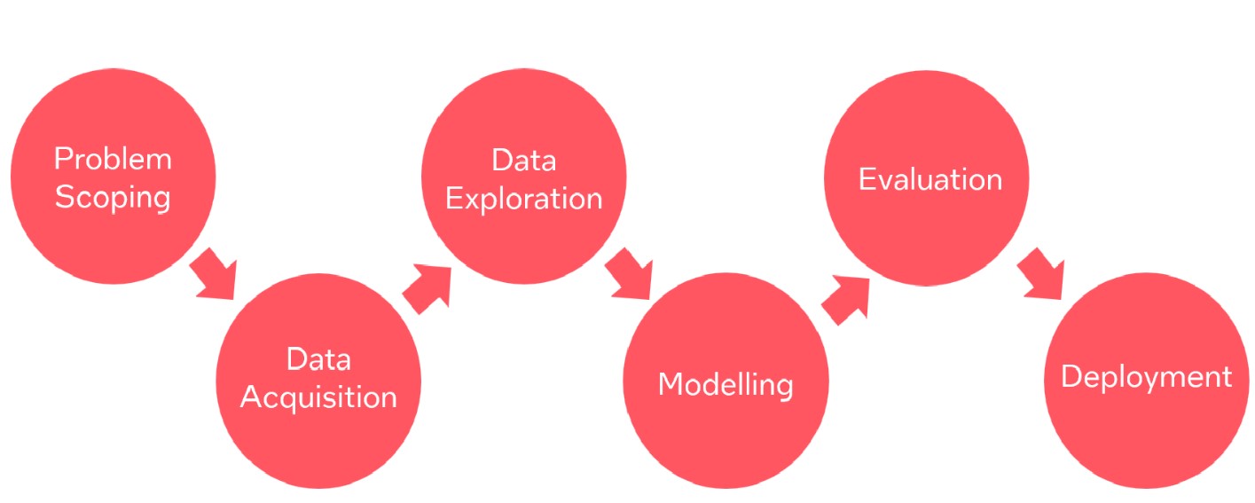 

Context: Understanding the Problem Statement --------Problem Scoping (AI Project Cycle - Step 1)
An ML based predictive solution for Utility Asset Health Maintanence
Predictive asset maintenance solutions of huge scale typically require operating across multiple hardware architectures. Accelerating training for the ever-increasing size of datasets and machine learning models is a major challenge while adopting AI.
Industrial scenario for predictive asset maintenance, with huge set of batch processing, requires fast prediction time without accuracy lose.
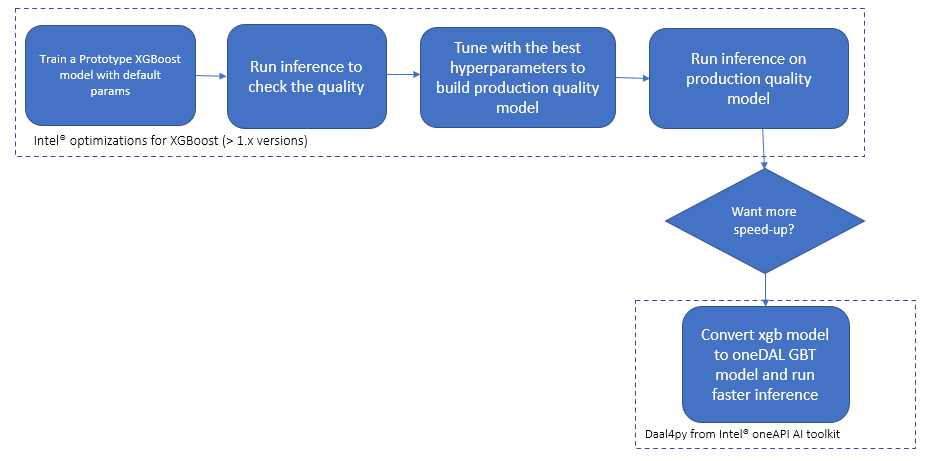
One of the important problem statement on this industrial scenario is to improve the MLOps time for developing and deploying new models due to its ever-increasing size of datasets over a period of time. XGBoost classifier with HIST tree method has been choosen to address this problem which will improve the overall training/tuning and validation time.
Import the useful Packages & Libraries
We import the necessary packages and libraries to get started.
Pandas - One of the most common packages used in machine learning for analysing data.
Numpy - Used to deal with numerical values and to perform mathematical expressions on arrays.
XGBoost - Used for classification and regression problems.
To learn more about Pandas click here, whereas for NumPy click here and for XGBoost click here.
%pip install ipython-autotime
%load_ext autotime
Requirement already satisfied: ipython-autotime in c:\Program Files\Python314\Lib\site-packages (0.3.2)
Requirement already satisfied: ipython in C:\Users\joann\AppData\Roaming\Python\Python314\site-packages (from ipython-autotime) (9.17.1)
Requirement already satisfied: colorama>=0.4.4 in C:\Users\joann\AppData\Roaming\Python\Python314\site-packages (from ipython->ipython-autotime) (0.4.6)
Requirement already satisfied: ipython-pygments-lexers>=1.0.0 in C:\Users\joann\AppData\Roaming\Python\Python314\site-packages (from ipython->ipython-autotime) (1.1.1)
Requirement already satisfied: jedi>=0.18.2 in C:\Users\joann\AppData\Roaming\Python\Python314\site-packages (from ipython->ipython-autotime) (0.20.0)
Requirement already satisfied: matplotlib-inline>=0.1.6 in C:\Users\joann\AppData\Roaming\Python\Python314\site-packages (from ipython->ipython-autotime) (0.2.2)
Requirement already satisfied: prompt_toolkit<3.1.0,>=3.0.41 in C:\Users\joann\AppData\Roaming\Python\Python314\site-packages (from ipython->ipython-autotime) (3.0.53)
Requirement already satisfied: psutil>=7 in C:\Users\joann\AppData\Roaming\Python\Python314\site-packages (from ipython->ipython-autotime) (7.2.2)
Requirement already satisfied: pygments>=2.14.0 in C:\Users\joann\AppData\Roaming\Python\Python314\site-packages (from ipython->ipython-autotime) (2.21.0)
Requirement already satisfied: stack_data>=0.6.0 in C:\Users\joann\AppData\Roaming\Python\Python314\site-packages (from ipython->ipython-autotime) (0.6.3)
Requirement already satisfied: traitlets>=5.13.0 in C:\Users\joann\AppData\Roaming\Python\Python314\site-packages (from ipython->ipython-autotime) (5.16.1)
Requirement already satisfied: wcwidth>=0.1.4 in C:\Users\joann\AppData\Roaming\Python\Python314\site-packages (from prompt_toolkit<3.1.0,>=3.0.41->ipython->ipython-autotime) (0.9.2)
Requirement already satisfied: parso<0.9.0,>=0.8.6 in C:\Users\joann\AppData\Roaming\Python\Python314\site-packages (from jedi>=0.18.2->ipython->ipython-autotime) (0.8.7)
Requirement already satisfied: executing>=1.2.0 in C:\Users\joann\AppData\Roaming\Python\Python314\site-packages (from stack_data>=0.6.0->ipython->ipython-autotime) (2.2.1)
Requirement already satisfied: asttokens>=2.1.0 in C:\Users\joann\AppData\Roaming\Python\Python314\site-packages (from stack_data>=0.6.0->ipython->ipython-autotime) (3.0.2)
Requirement already satisfied: pure-eval in C:\Users\joann\AppData\Roaming\Python\Python314\site-packages (from stack_data>=0.6.0->ipython->ipython-autotime) (0.2.4)
Note: you may need to restart the kernel to use updated packages.
time: 108 μs (started: 2026-10-06 14:09:25 -07:00)
import pandas as pd
import time
import numpy as np
import xgboost as xgb
import pickle
from sklearn.model_selection import GridSearchCV
from sklearn.model_selection import train_test_split
from sklearn.preprocessing import RobustScaler


import warnings
warnings.filterwarnings("ignore")
time: 1.87 ms (started: 2026-10-06 14:09:25 -07:00)
Dataset: Data Acquisition (AI Project Cycle - Step 2)
The process of gathering accurate and reliable data to work with is known as data acquisition.
Four lists are created namely manufacturer_list, species_list, district_list and treatment_list. A variable called dsize has been initialized with a value of 25000
start = time.time()
dsize = 25000
print(f'Generating data with the size {dsize}')
np.random.seed(1)
manufacturer_list = ['A', 'B', 'C', 'D', 'E', 'F', 'G', 'H', 'I', 'J']
species_list = ['C1', 'C2', 'C3', 'C4', 'C5', 'C6', 'C7']
district_list = ['N', 'NE', 'NW', 'E', 'W', 'S', 'SE', 'SW']
treatment_list = ['Oil', 'Pentachlorophenol', 'Untreated', 'Creosote', 'UNK', 'Cellon']
Generating data with the size 25000
time: 2.89 ms (started: 2026-10-06 14:09:25 -07:00)
The below cell generates a dataframe having 10 columns and 25000 rows. Each column signifies a feature of the dataframe. The dsize variable has been used here to set the number of rows in the dataframe.
data = pd.DataFrame({"Age": np.random.choice(range(1, 101), dsize, replace=True),
                     "Elevation": np.random.randint(low=-300, high=4500, size=dsize),
                     "Pole_Height": np.random.normal(60, 15, size=dsize),
                     "Measured_Length": np.random.randint(low=1, high=2000, size=dsize),
                     "Manufacturer": np.random.choice(manufacturer_list, dsize, replace=True),
                     "Species": np.random.choice(species_list, dsize, replace=True),
                     "Number_Repairs": np.random.choice(range(1, 7), dsize, replace=True),
                     "District": np.random.choice(district_list, dsize, replace=True),
                     "Tele_Attached": np.random.choice(range(0, 2), dsize, replace=True),
                     "Original_Treatment": np.random.choice(treatment_list, dsize, replace=True)})
time: 22.6 ms (started: 2026-10-06 14:09:25 -07:00)
# changing Tele_Attatched into an object variable
print('changing Tele_Attatched into an object variable')
data[['Number_Repairs', 'Tele_Attached']] = data[['Number_Repairs', 'Tele_Attached']].astype('object')
changing Tele_Attatched into an object variable
time: 6.22 ms (started: 2026-10-06 14:09:25 -07:00)
# Generating our target variable Asset_Label
print('Generating our target variable Asset_Label')
data['Asset_Label'] = np.random.choice(range(0, 2), dsize, replace=True, p=[0.99, 0.01])
Generating our target variable Asset_Label
time: 4.99 ms (started: 2026-10-06 14:09:25 -07:00)
# Creating correlation between our variables and our target variable<br>
# When age is 60-70 and over 95 change Asset_Label to 1
print('Creating correlation between our variables and our target variable')
print('When age is 60-70 and over 95 change Asset_Label to 1')
data['Asset_Label'] = np.where(((data.Age > 0) & (data.Age <= 5)) | (data.Age > 45),
                               1, data.Asset_Label)
Creating correlation between our variables and our target variable
When age is 60-70 and over 95 change Asset_Label to 1
time: 4.7 ms (started: 2026-10-06 14:09:25 -07:00)
# When elevation is between 500-1500 change Asset_Label to 1
print('When elevation is between 500-1500 change Asset_Label to 1')
data['Asset_Label'] = np.where((data.Elevation >= -300) & (data.Elevation <= 1400),
                               1, data.Asset_Label)
When elevation is between 500-1500 change Asset_Label to 1
time: 4.27 ms (started: 2026-10-06 14:09:25 -07:00)
# When Manufacturer is A, E, or H change Asset_Label to have  95% 0's
print("When Manufacturer is A, E, or H change Asset_Label to have  95% 0's")
data['Temp_Var'] = np.random.choice(range(0, 2), dsize, replace=True, p=[0.95, 0.05])
data['Asset_Label'] = np.where((data.Manufacturer == 'A') |
                               (data.Manufacturer == 'E') |
                               (data.Manufacturer == 'H'),
                               data.Temp_Var,
                               data.Asset_Label)
When Manufacturer is A, E, or H change Asset_Label to have 95% 0's
time: 16.7 ms (started: 2026-10-06 14:09:25 -07:00)
# When Species is C2 or C5 change Asset_Label to have 90% to 0's
print("When Species is C2 or C5 change Asset_Label to have 90% to 0's")
data['Temp_Var'] = np.random.choice(range(0, 2), dsize, replace=True, p=[0.9, 0.1])
data['Asset_Label'] = np.where((data.Species == 'C2') | (data.Species == 'C5'),
                               data.Temp_Var,
                               data.Asset_Label)
When Species is C2 or C5 change Asset_Label to have 90% to 0's
time: 12.7 ms (started: 2026-10-06 14:09:25 -07:00)
# When District is NE or W change Asset_Label to have 90% to 0's
print("When District is NE or W change Asset_Label to have 90% to 0's")
data['Temp_Var'] = np.random.choice(range(0, 2), dsize, replace=True, p=[0.95, 0.05])
data['Asset_Label'] = np.where((data.District == 'NE') | (data.District == 'W'),
                               data.Temp_Var, data.Asset_Label)
When District is NE or W change Asset_Label to have 90% to 0's
time: 10.6 ms (started: 2026-10-06 14:09:25 -07:00)
# When District is Untreated change Asset_Label to have 70% to 1's
print("When District is Untreated change Asset_Label to have 70% to 1's")
data['Temp_Var'] = np.random.choice(range(0, 2), dsize, replace=True, p=[0.25, 0.75])
data['Asset_Label'] = np.where((data.Original_Treatment == 'Untreated'),
                               data.Temp_Var,
                               data.Asset_Label)
When District is Untreated change Asset_Label to have 70% to 1's
time: 9.83 ms (started: 2026-10-06 14:09:25 -07:00)
# When Age is greater than 90 and Elevaation is less than 1200
# and Original_treatment is Oil change Asset_Label to have 90% to 1's
print("When Age is greater than 90 and Elevaation is less than 1200 \nand Original_treatment is Oil change Asset_Label to have 90% to 1's")
data['Temp_Var'] = np.random.choice(range(0, 2), dsize, replace=True, p=[0.05, 0.95])
data['Asset_Label'] = np.where((data.Age >= 20) &
                               (data.Elevation <= 1000) &
                               (data.Original_Treatment == 'Oil') &
                               (data.Pole_Height >= 60),
                               data.Temp_Var,
                               data.Asset_Label)
When Age is greater than 90 and Elevaation is less than 1200
and Original_treatment is Oil change Asset_Label to have 90% to 1's
time: 7.19 ms (started: 2026-10-06 14:09:25 -07:00)
#The label'Temp_Var' is being removed using the drop function.
data.drop('Temp_Var', axis=1, inplace=True)
time: 2.61 ms (started: 2026-10-06 14:09:25 -07:00)
Categorical_Variables = pd.get_dummies(
                           data[[
                               'Manufacturer',
                               'District',
                               'Species',
                               'Original_Treatment']],
                           drop_first=True)
data = pd.concat([data, Categorical_Variables], axis=1)
data.drop(['Manufacturer', 'District', 'Species', 'Original_Treatment'], axis=1, inplace=True)

data = data.astype({'Tele_Attached': 'int32', 'Number_Repairs': 'float64'})

etime = time.time() - start
datasize = data.shape
print(f"=====> Time taken {etime} secs for data generation for the size of {datasize}")
=====> Time taken 0.302173376083374 secs for data generation for the size of (25000, 34)
time: 34.9 ms (started: 2026-10-06 14:09:25 -07:00)
View the data
#Prints the first five entry of the dataframe
data.head()time: 23.3 ms (started: 2026-10-06 14:09:25 -07:00)
Data Preprocessing ------ Data Exploration(AI Project Cycle - Step 3)
View the information of data
Data exploration is performed to gather information on data and based on the gaind insights, various pre-processing functions are implemented.
The general insights that are obtained from data exploration are
1.Statistical information of the entire data
2.Outliers present in the data
3.Datatypes
4.Null values
# info() helps summarize the dataset- It gives basic information like number of non-null values, datatypes and memory usage
# It is a good practise to start by this information
data.info()
<class 'pandas.DataFrame'>
RangeIndex: 25000 entries, 0 to 24999
Data columns (total 34 columns):
# Column Non-Null Count Dtype
--- ------ -------------- -----
0 Age 25000 non-null int64
1 Elevation 25000 non-null int32
2 Pole_Height 25000 non-null float64
3 Measured_Length 25000 non-null int32
4 Number_Repairs 25000 non-null float64
5 Tele_Attached 25000 non-null int32
6 Asset_Label 25000 non-null int64
7 Manufacturer_B 25000 non-null bool
8 Manufacturer_C 25000 non-null bool
9 Manufacturer_D 25000 non-null bool
10 Manufacturer_E 25000 non-null bool
11 Manufacturer_F 25000 non-null bool
12 Manufacturer_G 25000 non-null bool
13 Manufacturer_H 25000 non-null bool
14 Manufacturer_I 25000 non-null bool
15 Manufacturer_J 25000 non-null bool
16 District_N 25000 non-null bool
17 District_NE 25000 non-null bool
18 District_NW 25000 non-null bool
19 District_S 25000 non-null bool
20 District_SE 25000 non-null bool
21 District_SW 25000 non-null bool
22 District_W 25000 non-null bool
23 Species_C2 25000 non-null bool
24 Species_C3 25000 non-null bool
25 Species_C4 25000 non-null bool
26 Species_C5 25000 non-null bool
27 Species_C6 25000 non-null bool
28 Species_C7 25000 non-null bool
29 Original_Treatment_Creosote 25000 non-null bool
30 Original_Treatment_Oil 25000 non-null bool
31 Original_Treatment_Pentachlorophenol 25000 non-null bool
32 Original_Treatment_UNK 25000 non-null bool
33 Original_Treatment_Untreated 25000 non-null bool
dtypes: bool(27), float64(2), int32(3), int64(2)
memory usage: 1.7 MB
time: 12.9 ms (started: 2026-10-06 14:09:25 -07:00)
The describe() function gives the numerical statistical information of the dataframe
count - The number of non-empty values.
mean - The average value
std - The standard deviation
min - the minimum value
25% - The 25% percentile
50% - The 50% percentile
75% - The 75% percentile
max - the maximum value
data.describe()time: 40.1 ms (started: 2026-10-06 14:09:25 -07:00)
Find the total number of missing values feature wise
#It returns the number of null values in the dataframe for every column feature
#Using info() we can view the number of non-null values whereas isnull() gives the number of null values
data.isnull().sum()time: 12.2 ms (started: 2026-10-06 14:09:25 -07:00)
Splitting dataset into separate training and test set
The sklearn train_test_split method has been used to split the dataset into train and test cohorts. Here, 25% of the data has been allocated as test data. Since, Asset_Label has been removed from the overall data(X) and y has only one feature which is Asset_Label as the target variable.
datasize = data.shape

start = time.time()
X = data.drop('Asset_Label', axis=1)
y = data.Asset_Label

# original split .25
X_train, X_test, y_train, y_test = train_test_split(X, y, test_size=.25)

df_num_train = X_train.select_dtypes(['float', 'int', 'int32'])
df_num_test = X_test.select_dtypes(['float', 'int', 'int32'])
time: 22.5 ms (started: 2026-10-06 14:09:25 -07:00)
Scaling the data
We are performing scaling here to normalize the data within a sepcific range.
RobustScaler() uses interquartile range(IQR) and median is used to scale the data.
to know more about Roburst Scaler click here
robust_scaler = RobustScaler()
X_train_scaled = robust_scaler.fit_transform(df_num_train)
X_test_scaled = robust_scaler.transform(df_num_test)
time: 27.4 ms (started: 2026-10-06 14:09:25 -07:00)
# Making them pandas dataframes
X_train_scaled_transformed = pd.DataFrame(X_train_scaled,
                                          index=df_num_train.index,
                                          columns=df_num_train.columns)
X_test_scaled_transformed = pd.DataFrame(X_test_scaled,
                                         index=df_num_test.index,
                                         columns=df_num_test.columns)

del X_train_scaled_transformed['Number_Repairs']
del X_train_scaled_transformed['Tele_Attached']

del X_test_scaled_transformed['Number_Repairs']
del X_test_scaled_transformed['Tele_Attached']
time: 4.27 ms (started: 2026-10-06 14:09:25 -07:00)
# Dropping the unscaled numerical columns
X_train = X_train.drop(['Age', 'Elevation', 'Pole_Height', 'Measured_Length'], axis=1)
X_test = X_test.drop(['Age', 'Elevation', 'Pole_Height', 'Measured_Length'], axis=1)
time: 4.13 ms (started: 2026-10-06 14:09:25 -07:00)
# Creating train and test data with scaled numerical columns
X_train_scaled_transformed = pd.concat([X_train_scaled_transformed, X_train], axis=1)
X_test_scaled_transformed = pd.concat([X_test_scaled_transformed, X_test], axis=1)
time: 2.12 ms (started: 2026-10-06 14:09:25 -07:00)
#len(dataframe)returns the no of rows in the dataframe
len(X_train_scaled_transformed)18750time: 3.87 ms (started: 2026-10-06 14:09:25 -07:00)
len(X_test_scaled_transformed)6250time: 20.6 ms (started: 2026-10-06 14:09:25 -07:00)
#Prints the first five entry of the dataframe
X_train_scaled_transformed.head()time: 28.8 ms (started: 2026-10-06 14:09:26 -07:00)
#Prints the first five entry of the dataframe
X_test_scaled_transformed.head()time: 26.1 ms (started: 2026-10-06 14:09:26 -07:00)
y_train.head()time: 14.3 ms (started: 2026-10-06 14:09:26 -07:00)
Building a Model ------ Modeling ( AI Project Cycle - Step 4)
We will now use the XGBoost library to build the model. We will begin by defining the hyperparameters to make the ensemble model robust.
A powerful machine-learning algorithm called XGBoost can assist you in comprehending your data and taking wiser decisions.
An application of gradient-boosting decision trees is XGBoost. Data scientists and researchers from all around the world have utilised it to enhance their machine-learning models.
To know more about XGBoost click here
cv_val = 2
tuning = 1
TUNING = False
if tuning == "1":
    TUNING = True

def fit_xgb_model(x_data, y_data):
    """Use a XGBClassifier for this problem."""
    # prepare data for xgboost training
    dtrain = xgb.DMatrix(x_data, y_data)
    label = dtrain.get_label()
    ratio = float(np.sum(label == 0)) / np.sum(label == 1)
    # Set xgboost parameters
    parameters = {'scale_pos_weight': ratio.round(2), 'tree_method': 'hist'}

    # define the model to use
    if TUNING is False:
        xg_cl = xgb.XGBClassifier(use_label_encoder=False)
    else:
        xg_cl = xgb.XGBClassifier(use_label_encoder=False, eval_metric='logloss')
    xg_cl.set_params(**parameters)
    # Train the model
    xg_cl.fit(x_data, y_data)
    return xg_cl
time: 2.93 ms (started: 2026-10-06 14:09:26 -07:00)
X_train_scaled_transformed = X_train_scaled_transformed.astype(
                                {'Tele_Attached': 'float64',
                                 'Number_Repairs': 'float64'})
X_test_scaled_transformed = X_test_scaled_transformed.astype(
                                {'Tele_Attached': 'float64',
                                 'Number_Repairs': 'float64'})
time: 299 ms (started: 2026-10-06 14:09:26 -07:00)
What are Hyperparameters? • A hyperparameter is a parameter whose value is set before the learning process begins
• Algorithm hyperparameters affect the speed and quality of the learning process
• Hyperparameters are important because they can have a direct impact on the behaviour of the training algorithm and have a
significant impact on the performance of the model being trained
Examples - Number of epochs, number of clusters, batch size etc
Performing hyperparameter tuning
As shown below, we are trying to find which algorithm should be used to build the model and which hyperparameters would contribute to better performance:
In this case, C(adds penalty to each misclassified point) and kernel are the hyperparameters of SVM
n_estimators(this specifies the number of trees you want to build before taking the maximum voting or averages of predictions. Higher number of trees give you better performance but makes your code slower) - hyperparameter for random forest
C(logistic regression) large values of C give more freedom to the model. Conversely, smaller values of C constrain the model more
Training the Ensemble Model
XGBoost model has been fitted and the training time is checked.
Random search is used to select the best possible set of hyperparameters by creating a dictionary called ‘params’.
# Training
tstart = time.time()
xgb_model = fit_xgb_model(X_train_scaled_transformed, y_train)
ttime = time.time() - tstart
if TUNING is True:
    # GridSearchCV
    def timer(start_time=None):  # pylint: disable=missing-function-docstring
        if not start_time:
            start_time = datetime.now()
            return start_time
        if start_time:
            thour, temp_sec = divmod((datetime.now() - start_time).total_seconds(), 3600)
            tmin, tsec = divmod(temp_sec, 60)
            print(f'Time taken: {thour} hours {tmin} minutes and {round(tsec, 2)} seconds.')
        return 0

    # Hyper parameters for tuning
    params = {
        'min_child_weight': [1, 5, 10],
        'gamma': [0.5, 1, 1.5, 2, 5],
        # 'subsample': [0.6, 0.8, 1.0],
        # 'colsample_bytree': [0.6, 0.8, 1.0],
        'max_depth': [3, 4, 5],
        # 'learning_rate': [0.001, 0.01]
        }

    # n_jobs should be used according to the underlying HW accelerators, hence -1 is given
    random_search = GridSearchCV(xgb_model, param_grid=params, cv=cv_val, verbose=10, n_jobs=-1)

    # Here we go
    starttime = timer(None)  # timing starts from this point for "starttime" variable
    random_search.fit(X_train_scaled_transformed, y_train)
    timer(starttime)
time: 462 ms (started: 2026-10-06 14:09:26 -07:00)
Evaluating the Model ------- Evaluation (AI Project Cycle - Step 5)
By feeding the test dataset into the model and comparing the outputs with actual solutions, evaluation is a procedure for determining the dependability of any AI model based on outputs.
Testing the Ensemble Model
# XGBoost vanilla prediction (for accuracy comparison)
dtest = xgb.DMatrix(X_test_scaled_transformed, y_test)
pstart = time.time()
xgb_prediction = xgb_model.predict(X_test_scaled_transformed)
ptime = time.time() - pstart
xgb_errors_count = np.count_nonzero(xgb_prediction - np.ravel(y_test))

xgb_total = ptime

y_test = np.ravel(y_test)

etime = time.time() - start
accuracy_scr = 1 - xgb_errors_count / xgb_prediction.shape[0]
print(f'=====> Time taken {etime} secs for training and prediction for the data size of {datasize}')
print(f'=====> Training Time {ttime} secs')
print(f'=====> Prediction Time {ptime} secs')
print(f'=====> XGBoost accuracy score {accuracy_scr}')


print(f'\nOn predicting the test data using XGBoost algorithm, an accuaracy of {accuracy_scr*100}% and a training time of {ttime} seconds has been achieved. ')
=====> Time taken 1.1936328411102295 secs for training and prediction for the data size of (25000, 34)
=====> Training Time 0.4594869613647461 secs
=====> Prediction Time 0.021214723587036133 secs
=====> XGBoost accuracy score 0.9192
On predicting the test data using XGBoost algorithm, an accuaracy of 91.92% and a training time of 0.4594869613647461 seconds has been achieved.
time: 45.6 ms (started: 2026-10-06 14:09:26 -07:00)