Order to Delivery (OTD) Time Forecasting
Ease of e-commerce over the last decade, along with the recent COVID-19 pandemic, has seen a marked shift in consumer behavior and expectations when it comes to purchase - and more importantly, the delivery of goods. This has caused a paradigm shift in functioning of the supply chain. Along with delivery speed, consumers feel that the transparency around delivery time and shipment status are an equally important aspect of the fulfilment process. This has direct implications in customer churn/retention. More than half of consumers are less likely to shop with a retailer if the item is not delivered within 2 days of date promised. (source)
Order to Delivery Time Forecasting as a Supply Chain Optimization Usecase:
OTD forecasting is a key aspect of supply chain optimization as it helps to ensure that customers receive their products in a timely manner, it enables companies to make informed decisions about inventory, logistics and production which in turn helps to improve the overall efficiency of the supply chain.
AI Project Cycle 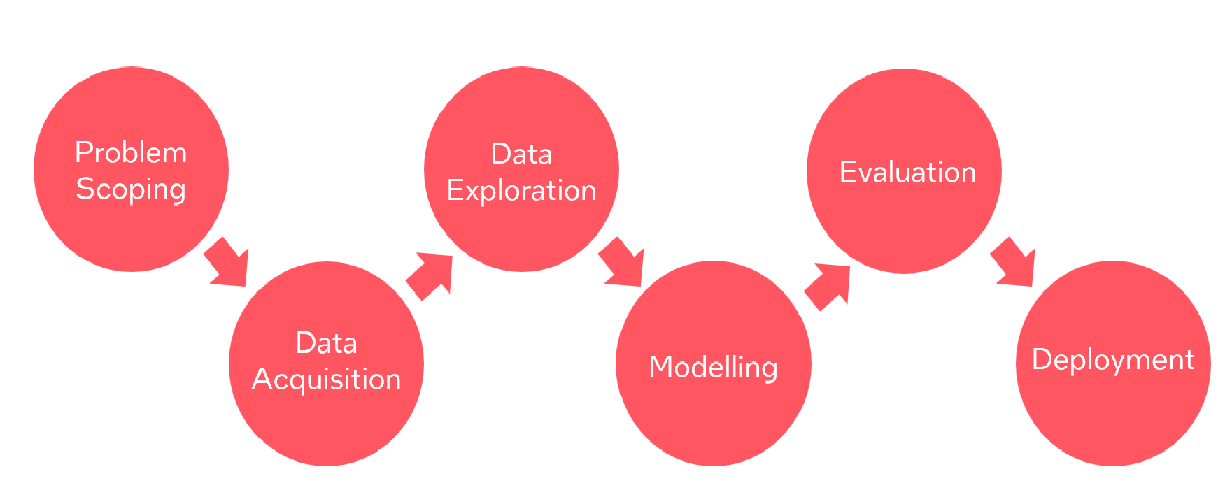 

Context: Understanding the Problem Statement --------Problem Scoping (AI Project Cycle - Step 1)
An ML based predictive solution for providing delivery time forecasting
An ML based predictive solution for providing delivery time forecasting can provide great insights to e-commerce platforms. From a customer-facing point of view these insights would help e-commerce platforms to give more accurate delivery forecasts to customers and decrease customer churn. In addition, the ML based predictive solution will also allow e-commerce platforms to take pre-emptive actions to mitigate delays, costs, and loss of revenue.
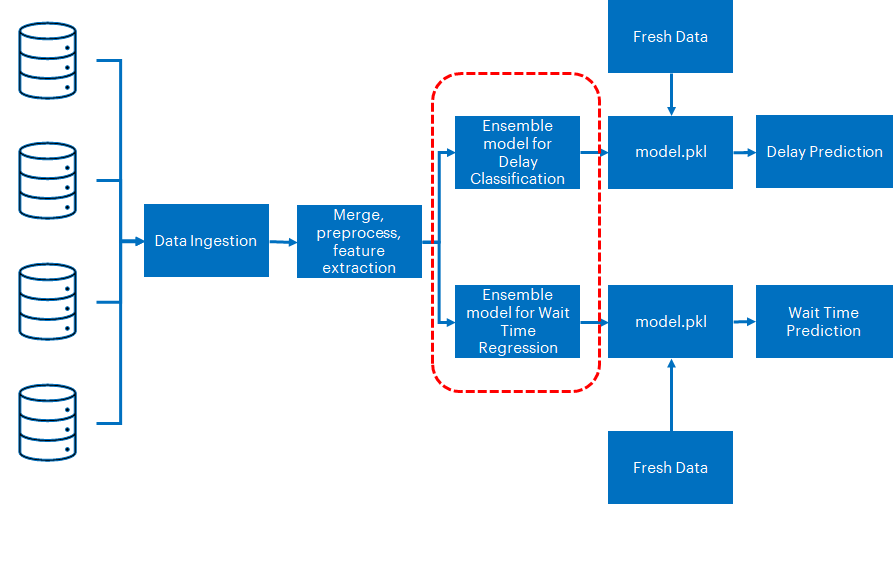
For the individual components of the ensemble model, we will use XGB, RF and SVM. These components will then be fed to a Voting Model, which is an ensemble model that combines the individual predictions to provide a final, consensus prediction. The final consensus prediction can be (1) a prediction for a wait time for a package and (2) if a delay will occur.
Import the useful Packages & Libraries
%pip install ipython-autotime
%load_ext autotime
from math import radians, sin, cos, asin, sqrt
# This line imports specific functions from the math library that are used for calculating the haversine distance between two points on a globe.
import pandas as pd
# This line imports the Pandas library, which is a popular library for data manipulation and analysis.
from sklearn.preprocessing import LabelEncoder, StandardScaler
# This line imports the LabelEncoder and StandardScaler classes from the scikit-learn library, which are used for preprocessing data for machine learning models.
import time
# This line imports the time module, which is used for timing the execution of code
import numpy as np
# This line imports the NumPy library, which provides support for numerical computing with Python.To know more about math click here
To know more about pandas click here
To know more about Sklearn’ Preprocessing package click here
To know more about time click here
To know more about numpy click here
Dataset: Data Acquisition (AI Project Cycle - Step 2)
Dataset downloading steps
DataSet: https://
“brazilian-ecommerce.zip” will get downloaded in the current data folder folderd
In the data folder execute the following command to unzip (Note: You may need to install unzip using: sudo apt-get install unzip)
unzip brazilian-ecommerce.zip
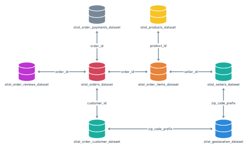
Source - Before we delve into the proposed architecture of the solution pipeline, it is critical to understand the dataset and its schema. The dataset consists of real-world delivery details sourced from a Brazilian E-commerce Company which was scrubbed and anonymized. It can be found here.
It consists of multiple tables which include relevant information about the customer, seller, order, location etc. The individual tables are interconnected as shown in the following schema. Relevant features will be extracted/designed from this data and then be used to train our supervised ML model.
Load/Read the Dataset
orders = pd.read_csv("./data/olist_orders_dataset.csv")
# This line reads the CSV file "olist_orders_dataset.csv" located in the "./data/" directory and stores its contents as a Pandas DataFrame named "orders".

items = pd.read_csv("./data/olist_order_items_dataset.csv")
# This line reads the CSV file "olist_order_items_dataset.csv" located in the "./data/" directory and stores its contents as a Pandas DataFrame named "items".

customers = pd.read_csv("./data/olist_customers_dataset.csv")
# This line reads the CSV file "olist_customers_dataset.csv" located in the "./data/" directory and stores its contents as a Pandas DataFrame named "customers".

'''
Your Code Here
'''
# This line reads the CSV file "olist_sellers_dataset.csv" located in the "./data/" directory and stores its contents as a Pandas DataFrame named "sellers".

'''
Your Code Here
'''
# This line reads the CSV file "olist_geolocation_dataset.csv" located in the "./data/" directory and stores its contents as a Pandas DataFrame named "geo".

'''
Your Code Here
'''
# This line reads the CSV file "olist_products_dataset.csv" located in the "./data/" directory and stores its contents as a Pandas DataFrame named "products".
View the data
orders.head()

# The code above assumes that a Pandas DataFrame named orders has been previously defined, and calls the head() method on that DataFrame.

# The head() method is used to display the first few rows of a DataFrame, by default the first five rows. This can be useful for quickly checking the structure and content of a DataFrame.

# So, this line of code will output the first five rows of the orders DataFrame, assuming it has been previously defined.
'''
Your Code Here
''''''
Your Code Here
''''''
Your Code Here
'''From a business perspective, we need to tackle two main challenges to ensure transparency for the customer:
Extracting insights/estimates into forecasted delivery
Increasing the accuracy of those insights and estimates
We can achieve the first objective by implementing multiple pipelines with separate objectives and the second one by utilizing techniques such as ensemble modeling to increase the accuracy of stand-alone ML components.
**A schematic of the proposed reference architecture is shown in the following figure. We start off with Data Ingestion from the multiple tables of the dataset, followed by merging and preprocessing for feature extraction. We can use the features to extract delivery insights in the form of predicted wait time as well as likelihood of delivery delay.
The former is a regression problem and the latter is a classification problem.
Data Preprocessing ------ Data Exploration(AI Project Cycle - Step 3)
View the information of data
# info() helps summarize the dataset- It gives basic information like number of non-null values, datatypes and memory usage
# It is a good practise to start by this information
products.info() '''
Your Code Here
''''''
Your Code Here
''''''
Your Code Here
'''Merge/Clean Data
To know more about how pandas dataframe merge function works click here
# Get the seller zip code of each order
middle = items[['order_id', 'seller_id']]
# This line creates a new dataframe middle that contains only the order_id and seller_id columns from the items dataframe.
middle_2 = middle.merge(sellers[['seller_id', 'seller_zip_code_prefix']], on="seller_id", how="outer")
# This line merges the middle dataframe with the seller_id and seller_zip_code_prefix columns from the sellers dataframe, creating a new dataframe middle_2. The outer join type is used, which means that all rows from both dataframes are included in the merged dataframe, and missing values are filled with NaN.
orders = orders.merge(middle_2, on="order_id", how="left")
# This line merges the orders dataframe with the middle_2 dataframe on the order_id column, creating a new orders dataframe. The left join type is used, which means that all rows from the orders dataframe are included in the merged dataframe, and missing values from the middle_2 dataframe are filled with NaN.
orders.head()# Get customer zip code of each order
orders = orders.merge(customers[['customer_id', 'customer_zip_code_prefix']],
on='customer_id', how="left")
# The code above performs a left merge operation between two Pandas dataframes named "orders" and "customers" using the "customer_id" column as the joining key. It then selects the "customer_id" and "customer_zip_code_prefix" columns from the "customers" dataframe and merges them with the "orders" dataframe based on the matching "customer_id" column.
orders.head()# Clean geo df
geo = geo[~geo['geolocation_zip_code_prefix'].duplicated()]
'''
This line first selects the 'geolocation_zip_code_prefix' column from the 'geo' DataFrame using the indexing operator []. The duplicated() method is then called on this column to create a boolean mask of rows that have duplicate values in this column.
The tilde operator (~) is used to invert this boolean mask, so that the mask contains True for rows that do not have duplicate values in this column.
'''
geo.head()# add seller coordinates to the orders
'''
Your Code Here
'''
# The code above performs a left join of two dataframes - "orders" and "geo" - using the "seller_zip_code_prefix" column of the "orders" dataframe and the "geolocation_zip_code_prefix" column of the "geo" dataframe as the join keys.
orders.head()# add customer coordinates to the orders
orders = orders.merge(geo, left_on="customer_zip_code_prefix",
right_on="geolocation_zip_code_prefix", how="left",
suffixes=("_seller", "_customer"))
# This code merges two Pandas DataFrames, orders and geo, on a common column, customer_zip_code_prefix in orders and geolocation_zip_code_prefix in geo. The resulting merged DataFrame contains all the columns from both DataFrames.# Clean orders
# 1-Filter out orders with multiple sellers Because each order only has one delivery date
df = orders.groupby(by="order_id").nunique()
# Groups the orders by order_id and calculates the number of unique values in each group using the nunique() method.
mono_orders = pd.Series(df[df['seller_id'] == 1].index)
# Selects the indices of the resulting DataFrame where the seller_id column equals 1 and stores them in a Pandas Series called mono_orders.
filtered_orders = orders.merge(mono_orders, how='inner')
# Merges the original orders DataFrame with mono_orders based on the order_id column using an inner join and stores the resulting DataFrame in a variable called filtered_orders.# 2-drop rows with missing values
filtered_orders = filtered_orders.drop(columns=["order_approved_at"])
# This line drops the "order_approved_at" column from the filtered_orders DataFrame. This column is not necessary for the analysis being performed.
filtered_orders = filtered_orders.dropna()
# This line drops any rows in the filtered_orders DataFrame that contain missing values. This is a common data preprocessing step to ensure that the dataset is clean and complete.
filtered_orders.head()# Define Function to calculate distance
def haversine_distance(lon1, lat1, lon2, lat2):
"""
Compute distance between two pairs of (lat, lng)
"""
lon1, lat1, lon2, lat2 = map(radians, [lon1, lat1, lon2, lat2])
dlon = lon2 - lon1
dlat = lat2 - lat1
a = sin(dlat / 2) ** 2 + cos(lat1) * cos(lat2) * sin(dlon / 2) ** 2
return 2 * 6371 * asin(sqrt(a))
# This line defines a function called haversine_distance that takes four arguments: lon1, lat1, lon2, and lat2. These arguments represent the longitude and latitude coordinates of two points on the globe.def get_package_size(items, products):
# Get Package Size
df_tmp = items[['order_id', 'product_id']].merge(products[['product_id', 'product_length_cm', 'product_height_cm',
'product_width_cm', 'product_weight_g']],
on="product_id",
how="outer")
df_tmp.loc[:, "product_size_cm3"] = \
df_tmp['product_length_cm']*df_tmp['product_width_cm'] * df_tmp['product_height_cm']
orders_size_weight = df_tmp.groupby("order_id", as_index=False).sum()[['order_id', 'product_size_cm3',
'product_weight_g']]
return orders_size_weight
# The code above defines a function called get_package_size that takes two arguments: items and products, which are Pandas DataFrames containing information about products and the items ordered.def object_to_int(dataframe_series):
if dataframe_series.dtype == 'object':
# This line checks if the data type of the input dataframe_series is "object", which typically represents string or categorical data.
dataframe_series = LabelEncoder().fit_transform(dataframe_series)
# This line uses the LabelEncoder() method from the scikit-learn library to encode the string or categorical data as integers. This is a common preprocessing step in machine learning to convert non-numeric data into a format that can be used by algorithms. The fit_transform() method fits the encoder to the data and transforms it.
return dataframe_series#It gives the numerical statistical information of the dataframe
orders.describe()
'''
The code above applies the describe() method to a Pandas DataFrame called orders, which provides summary statistics of the data in the DataFrame. Here's a brief explanation of what each statistic means:
count: the number of non-missing values in each column
mean: the average value of each column
std: the standard deviation of each column
min: the minimum value of each column
25%: the first quartile of each column (25th percentile)
50%: the second quartile of each column (50th percentile, equivalent to the median)
75%: the third quartile of each column (75th percentile)
max: the maximum value of each column
The describe() method is useful for quickly getting an overview of the data in a DataFrame, including identifying potential outliers or unusual patterns in the data.
'''Find the total number of missing values feature wise
# It returns the number of null values in the dataframe for every column feature
# Using info() we can view the number of non-null values whereas isnull() gives the number of null values
orders.isnull().sum()Scaling the data
def scaling(X_train, X_test):
'''
The code above defines a function called scaling that performs feature scaling using the StandardScaler class from scikit-learn.
'''
sc_X = StandardScaler()
X_train_scaled = sc_X.fit_transform(X_train)
X_test_scaled = sc_X.fit_transform(X_test)
return X_train_scaled, X_test_scaledSplitting dataset into separate training and test set
def split_data(final_df, columns_for_train, columns_for_pred, i_flag):
'''
This function is a convenient way to split a DataFrame into training and testing sets for machine learning purposes. The i_flag parameter is used to avoid a warning message related to the NumPy library, and the columns_for_train and columns_for_pred parameters allow for flexible selection of features and target variables.
'''
if i_flag:
from sklearnex import patch_sklearn # pylint: disable=C0415, E0401
patch_sklearn()
from sklearn.model_selection import train_test_split # pylint: disable=C0415
x_train, x_test, y_train, y_test = train_test_split(final_df[columns_for_train], final_df[columns_for_pred],
test_size=0.3, random_state=42)
return x_train, x_test, y_train, y_testfiltered_orders['distance'] = filtered_orders.apply(lambda row: haversine_distance(row["geolocation_lng_seller"],
row["geolocation_lat_seller"],
row["geolocation_lng_customer"],
row["geolocation_lat_customer"],),
axis=1,)
# This line creates a new column in the filtered_orders DataFrame called "distance" by applying the haversine_distance function to calculate the distance between the seller and the customer for each row in the DataFrame.
orders_size_weight = get_package_size(items, products)
filtered_orders = filtered_orders.merge(orders_size_weight, on='order_id', how='left')
# These lines merge information about the package size and weight for each order from the items and products DataFrames into the filtered_orders DataFrame.
# process time columns
time_columns = ['order_purchase_timestamp', 'order_delivered_customer_date', 'order_estimated_delivery_date']
for column in time_columns:
filtered_orders.loc[:, column] = pd.to_datetime(filtered_orders[column])
# These lines convert several time-related columns in the filtered_orders DataFrame from string format to datetime format using the pd.to_datetime function.
filtered_orders.loc[:, "wait_time"] = (filtered_orders['order_delivered_customer_date'] -
filtered_orders['order_purchase_timestamp']).dt.days
filtered_orders.loc[:, "est_wait_time"] = (filtered_orders['order_estimated_delivery_date'] -
filtered_orders['order_purchase_timestamp']).dt.days
# These lines calculate the wait time and estimated wait time for each order in days, based on the difference between the purchase time and the delivered/estimated delivery time.
filtered_orders.loc[:, "purchase_dow"] = filtered_orders.order_purchase_timestamp.dt.dayofweek
filtered_orders.loc[:, "year"] = filtered_orders.order_purchase_timestamp.dt.year
filtered_orders.loc[:, "purchase_month"] = filtered_orders.order_purchase_timestamp.dt.month
# These lines extract the day of the week, year, and month from the order_purchase_timestamp column in the filtered_orders DataFrame.
final_df = filtered_orders[['purchase_dow', 'purchase_month', 'year', 'product_size_cm3', 'product_weight_g',
'geolocation_state_customer', 'geolocation_state_seller', 'distance',
'wait_time', 'est_wait_time']]
# This line creates a new DataFrame called final_df by selecting certain columns from the filtered_orders DataFrame.
final_df['delay'] = final_df['wait_time'] - final_df['est_wait_time']
final_df['delay'] = final_df['delay'] > 0
final_df['delay'] = final_df['delay'].astype(int)
# These lines calculate the delay time for each order and encode it as a binary variable indicating whether there was a delay or not.
final_df_enc = final_df.apply(lambda x: object_to_int(x))
# This line applies the object_to_int function to each column in the final_df DataFrame to convert categorical variables into integer format. The object_to_int function is not shown in the code provided, but it likely uses the LabelEncoder class from the scikit-learn library to perform the conversion.
final_df_enc.head()# Export the final_df_enc DataFrame to a CSV file
'''
Your Code Here
'''