Below, we have imported the Python libraries needed for this module. Run the code in this cell before running any other code cells, and be careful not to change any of the code. You can run the cell in any of these ways:

Ctrl + Enter: Run the cell and keep the cursor in the same cell.
Shift + Enter: Run the cell and move the cursor to the next cell.
Click the Play button: Click the Run (play) button to the left of the cell to execute it.

# Necessary imports for this module
from utils import *

Sampling Distributions & Central Limit Theorem¶

Estimated Time: 30 Minutes
Professor: Alice Martinez
Developers: James Geronimo, Mark Barranda, Rinrada Maneenop

The sampling distribution of a statistic is the distribution of all values of a statistic when all possible samples of the same size n are taken from the same population.

The basic idea is this: If you were to take multiple samples, what values from those samples will give you the best estimates of the population values?

Example 1: Fair Die¶

n_samples = 10000
sample_size = 5
population = np.arange(1, 7)

Means¶

Sampling Procedure:
Roll a fair six-sided die 5 times and record the sample mean, $\bar{x}$ .
Repeat this process 10,000 times to build a distribution of sample means.

Population Mean ( $\mu$ ): 3.5

🟩 The dashed green line represents the mean of all sample means.

fair_die_means(n_samples, sample_size, population)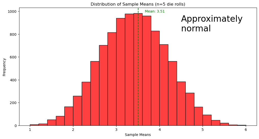

In this cell block, we show a few indivudal sample means generate from five samples.

for i in range(5):
    rolls = np.random.choice(population, size=sample_size)
    print(f"Sample {i+1} rolls: {rolls}, Sample Mean: {np.mean(rolls):.2f}")

Sample 1 rolls: [4 1 4 2 5], Sample Mean: 3.20
Sample 2 rolls: [6 3 1 1 6], Sample Mean: 3.40
Sample 3 rolls: [3 4 3 5 2], Sample Mean: 3.40
Sample 4 rolls: [3 3 2 6 1], Sample Mean: 3.00
Sample 5 rolls: [6 5 6 3 3], Sample Mean: 4.60

All outcomes are equally likely so the population mean is 3.5.

The mean of the sample means in 10,000 trials is 3.51. If continued indefinitely, the sample mean will be 3.5.

Note:

The mean of the sample means equals the value of the population mean
The sample means have a approximately normal distribution

Variances¶

Sampling Procedure:
Roll a fair six-sided die 5 times and record the sample variance, $s^2$ .
Repeat this process 10,000 times to build a distribution of sample variances.

Population Variance ( $\sigma^2$ ): 2.9

🟩 The dashed green line represents the mean of all sample variances.

fair_die_variances(n_samples, sample_size, population)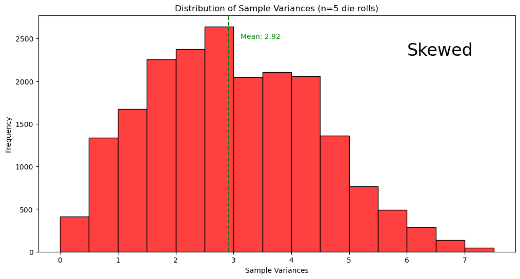

In this cell block, we show a few individual sample variances generate from five samples.

for i in range(5):
    rolls = np.random.choice(population, size=sample_size)
    print(f"Sample {i+1} rolls: {rolls}, Sample Mean: {np.var(rolls, ddof=1):.2f}")

Sample 1 rolls: [4 3 4 1 3], Sample Mean: 1.50
Sample 2 rolls: [1 4 4 2 6], Sample Mean: 3.80
Sample 3 rolls: [1 1 5 5 5], Sample Mean: 4.80
Sample 4 rolls: [5 1 2 5 1], Sample Mean: 4.20
Sample 5 rolls: [2 2 5 1 3], Sample Mean: 2.30

All outcomes are equally likely so the population variance is 2.9.

The mean of sample variance in the 10,000 trials is 2.92. If continued indefinitely, the sample variance will be 2.9.

Note:

The mean of the sample variances equals the value of the population variance
The sample variances have a skewed distribution

Proportions¶

Sampling Procedure:
Roll a fair six-sided die 5 times and record the proportion of odd numbers.
Repeat this process 10,000 times to build a distribution of odd number proportions.

Population Proportion of Odd Numbers ( $p$ ): 0.5
$\hat{p}$ represents the sample proportion of odd numbers

🟩 The dashed green line represents the mean of all odd number proportions.

fair_die_proportions(n_samples, sample_size, population)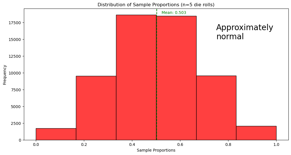

In this cell block, we show a few indivudal sample proportions generate from five samples.

for i in range(5):
    rolls = np.random.choice(population, size=sample_size)
    print(f"Sample {i+1} rolls: {rolls}, Sample Mean: {np.sum(rolls % 2 == 1) / sample_size:.2f}")

Sample 1 rolls: [3 6 6 3 5], Sample Mean: 0.60
Sample 2 rolls: [4 6 4 1 3], Sample Mean: 0.40
Sample 3 rolls: [3 4 6 1 2], Sample Mean: 0.40
Sample 4 rolls: [3 5 4 1 3], Sample Mean: 0.80
Sample 5 rolls: [6 1 5 1 4], Sample Mean: 0.60

All outcomes are equally likely so the population proportion of odd numbers is 0.5.

The mean of the sample proportions of the 10,000 trials is 0.503. If continued indefinitely, the mean of sample proportions will be 0.5.

Note:

The mean of the sample proportions equals the value of the population proportions
The sample proportions have a approximately normal distribution

Estimators¶

Using the above information, we discover biased and unbiased estimators of population parameters.

Unbiased Estimators:¶

The sample mean $\bar{x}$ , sample variance $s^2$ , and sample proportion $\hat{p}$ of the samples are unbiased estimators of the corresponding population parameters $\mu$ , $\sigma^2$ , and $p$ because they target the value that the population would have.

Biased Estimators:¶

The sample median, sample range, and sample standard deviation $s$ do NOT target their corresponding population parameters, so they are generally NOT good estimators. However: often bias in the $s$ is small enough that it is used to estimate $\sigma$ .

Example 2: Assassinated Presidents¶

There are four U.S. presidents who were assassinated in office. Their ages (in years) were Lincoln 56, Garfield 49, McKinley 58, and Kennedy 46.

a) Assuming that 2 of the ages are randomly selected with replacement from [56, 49, 58, 46], list the 16 different possible samples by replacing the ellipses with appropriate values. We’ve filled out a few as a hint:

[56, 56] [49, 56] [58, 56] [46, 56]
[56, 49] [49, 49] [58, 49] [46, 49]
[56, 58] [49, 58] [58, 58] [46, 58]
[56, 46] [49, 46] [58, 46] [46, 46]

b) Find the sample mean and range of possible samples by completing the functions calculate_mean, calculate_range, and calculate_probability. Then, run the cell to create tables that represent the probability distribution of each statistic.

def calculate_mean(number1, number2):
    """Calculate the mean of two numbers."""
    return (number1 + number2) / 2
    
def calculate_range(number1, number2):
    """Calculate the range of two numbers."""
    return max(number1, number2) - min(number1, number2)

def calculate_probability(frequency, total_samples):
    """Calculate the probability given frequency and total_samples."""
    return frequency / total_samples

mean_range_tables(calculate_mean, calculate_range, calculate_probability)

Calculated Sample Means and Ranges:
Sample: [56, 56], Mean: 56.0, Range: 0
Sample: [56, 49], Mean: 52.5, Range: 7
Sample: [56, 58], Mean: 57.0, Range: 2
Sample: [56, 46], Mean: 51.0, Range: 10
Sample: [49, 56], Mean: 52.5, Range: 7
Sample: [49, 49], Mean: 49.0, Range: 0
Sample: [49, 58], Mean: 53.5, Range: 9
Sample: [49, 46], Mean: 47.5, Range: 3
Sample: [58, 56], Mean: 57.0, Range: 2
Sample: [58, 49], Mean: 53.5, Range: 9
Sample: [58, 58], Mean: 58.0, Range: 0
Sample: [58, 46], Mean: 52.0, Range: 12
Sample: [46, 56], Mean: 51.0, Range: 10
Sample: [46, 49], Mean: 47.5, Range: 3
Sample: [46, 58], Mean: 52.0, Range: 12
Sample: [46, 46], Mean: 46.0, Range: 0


---Probability Distribution of Sample Mean ---
| Sample Mean (x̄) | Frequency | Probability P(x̄) |
|-----------------+-----------+------------------|
| 46.00           | 1         | 0.0625           |
| 47.50           | 2         | 0.1250           |
| 49.00           | 1         | 0.0625           |
| 51.00           | 2         | 0.1250           |
| 52.00           | 2         | 0.1250           |
| 52.50           | 2         | 0.1250           |
| 53.50           | 2         | 0.1250           |
| 56.00           | 1         | 0.0625           |
| 57.00           | 2         | 0.1250           |
| 58.00           | 1         | 0.0625           |
Mean of Sample Means: 52.25


--- Probability Distribution of Sample Range ---
| Sample Range (R) | Frequency | Probability P(R) |
|------------------+-----------+------------------|
| 0.00             | 4         | 0.2500           |
| 2.00             | 2         | 0.1250           |
| 3.00             | 2         | 0.1250           |
| 7.00             | 2         | 0.1250           |
| 9.00             | 2         | 0.1250           |
| 10.00            | 2         | 0.1250           |
| 12.00            | 2         | 0.1250           |
Mean of Sample Ranges: 5.375

c) Calculate the population_mean and population_range. Then, for each statistic, compare the mean of sample statistics to the population statistic. Which sampling distributions target the population parameter?

population_ages = [56, 49, 58, 46]
population_mean = np.mean(population_ages)
population_range = max(population_ages) - min(population_ages)

print(f"Population Mean: {population_mean}")
print(f"Population Range: {population_range}")

Population Mean: 52.25
Population Range: 12

Mean of sample means equals the population mean which makes this a unbiased estimator

Mean of sample ranges does not equal the population range which makes this a biased estimator

Standard Deviation and Variance¶

Variance measures how spread out the data are around the mean.
- For a population with values $x_1, x_2, \dots, x_N$ and mean $\mu$ :
  $\sigma^2 = \frac{1}{N} \sum_{i=1}^N (x_i - \mu)^2$
  (1)
- For a sample with values $x_1, x_2, \dots, x_n$ and sample mean $\bar{x}$ , the sample variance is:
  $s^2 = \frac{1}{n-1} \sum_{i=1}^n (x_i - \bar{x})^2$
  (2)
Standard deviation is the square root of the variance.
- For a population: $\sigma = \sqrt{\sigma^2}$
- For a sample: $s = \sqrt{s^2}$

It is in the same units as the original data and tells you a typical distance of values from the mean.

Below we compute the population variance and population standard deviation for the four ages (56, 49, 58, 46). Run this cell to see their values. When you code the sampling distribution in part (d), you can use this as a reference for the np.var and np.std syntax, and compare your sample statistics to these population parameters.

# The four ages (population)
population_ages = np.array([56, 49, 58, 46])

# Population variance and standard deviation (ddof=0 is the default for population)
population_variance = np.var(population_ages, ddof = 0)
population_std = np.std(population_ages, ddof = 0)

print(f"Population variance (σ²): {population_variance}")
print(f"Population standard deviation (σ): {population_std}")

Population variance (σ²): 24.1875
Population standard deviation (σ): 4.9180788932265

d) Find the sample standard deviation and variance of possible samples by completing the functions standard_deviation and variance. Then, run the cell to create tables that represent the probability distribution of each statistic.

Hint: Use ddof=1 in np.std and np.var for sample statistics; the default ddof=0 gives the population variance and standard deviation.

def standard_deviation(number1, number2):
    """Calculate the sample standard deviation of two numbers."""
    two_nums_array = np.array([number1, number2])
    return np.std(two_nums_array, ddof=1)

def variance(number1, number2):
    """Calculate the sample variance of two numbers."""
    two_nums_array = np.array([number1, number2])
    return np.var(two_nums_array, ddof=1)

std_var_tables(standard_deviation, variance)

Calculated Sample Standard Deviations and Variances:
Sample: [56, 56], Standard Deviation: 0.0, Variance: 0.0
Sample: [56, 49], Standard Deviation: 4.949747468305833, Variance: 24.5
Sample: [56, 58], Standard Deviation: 1.4142135623730951, Variance: 2.0
Sample: [56, 46], Standard Deviation: 7.0710678118654755, Variance: 50.0
Sample: [49, 56], Standard Deviation: 4.949747468305833, Variance: 24.5
Sample: [49, 49], Standard Deviation: 0.0, Variance: 0.0
Sample: [49, 58], Standard Deviation: 6.363961030678928, Variance: 40.5
Sample: [49, 46], Standard Deviation: 2.1213203435596424, Variance: 4.5
Sample: [58, 56], Standard Deviation: 1.4142135623730951, Variance: 2.0
Sample: [58, 49], Standard Deviation: 6.363961030678928, Variance: 40.5
Sample: [58, 58], Standard Deviation: 0.0, Variance: 0.0
Sample: [58, 46], Standard Deviation: 8.48528137423857, Variance: 72.0
Sample: [46, 56], Standard Deviation: 7.0710678118654755, Variance: 50.0
Sample: [46, 49], Standard Deviation: 2.1213203435596424, Variance: 4.5
Sample: [46, 58], Standard Deviation: 8.48528137423857, Variance: 72.0
Sample: [46, 46], Standard Deviation: 0.0, Variance: 0.0


---Probability Distribution of Sample Standard Deviation ---
| Sample Std Dev (s) | Frequency | Probability P(s) |
|--------------------+-----------+------------------|
| 0.0                | 4         | 0.2500           |
| 1.4142135623730951 | 2         | 0.1250           |
| 2.1213203435596424 | 2         | 0.1250           |
| 4.949747468305833  | 2         | 0.1250           |
| 6.363961030678928  | 2         | 0.1250           |
| 7.0710678118654755 | 2         | 0.1250           |
| 8.48528137423857   | 2         | 0.1250           |
Mean of Sample Standard Deviations: 3.8006989488776926


--- Probability Distribution of Sample Variance ---
| Sample Variance (s^2) | Frequency | Probability P(s^2) |
|-----------------------+-----------+--------------------|
| 0.0                   | 4         | 0.2500             |
| 2.0                   | 2         | 0.1250             |
| 4.5                   | 2         | 0.1250             |
| 24.5                  | 2         | 0.1250             |
| 40.5                  | 2         | 0.1250             |
| 50.0                  | 2         | 0.1250             |
| 72.0                  | 2         | 0.1250             |
Mean of Sample Variances: 24.1875

Complete each of the following expressions:

Mean of sample medians equals the population median which makes this a unbiased estimator

Mean of the sample proportions equals the population proportion, so it is an unbiased estimator

Mean of the sample variances equals the population variance, so it is an unbiased estimator

Mean of the sample standard deviations does not equal the population standard deviation, so it is a biased estimator

📋 Post-Notebook Reflection Form¶

Thank you for completing the notebook! We’d love to hear your thoughts so we can continue improving and creating content that supports your learning.

Please take a few minutes to fill out this short reflection form:

👉 Click here to fill out the Reflection Form

🧠 Why it matters:¶

Your feedback helps us understand:

How clear and helpful the notebook was
What you learned from the experience
How your views on data science may have changed
What topics you’d like to see in the future

This form is anonymous and should take less than 5 minutes to complete. We appreciate your time and honest input! 💬

Hurray! You have completed this notebook! 🚀