Hypothesis Testing with One Sample (Instructor — solutions filled in)

Estimated Time: 35–40 Minutes
Professor: Elizabeth Schwartz
Developers: Ariana Ghimire, Rinrada Maneenop
Textbook Reference: OpenStax Introductory Statistics 2e, Chapter 9 (Hypothesis Testing with One Sample)
Goal: Learn how to set up, run, and interpret one-sample hypothesis tests for a mean and a proportion.

Table of Contents¶

Quick Concepts and Setup
Null and Alternative Hypotheses
Type I and Type II Errors
The p-Value and Decision Rule
Test 1 — Population Mean (t-Test)
Test 2 — Population Proportion (z-Test)
Sandbox: Your Own Hypothesis Test

Notebook Structure¶

You will see short concept → example → practice cycles.

This instructor notebook includes completed code where the student version used ..., and staff answers for the early free-response prompts. For class, distribute hypothesis_testing.ipynb and keep this file private. Run cells in order from the top to verify output on your machine.

This notebook follows OpenStax Ch. 9 guidance:

Always state H₀ and Hₐ before computing anything.
Compare the p-value to α to make a decision.
Write a conclusion in plain English — not just “reject” or “fail to reject.”

1. Quick Concepts and Setup¶

1.1. Learning Objectives¶

Is the average NBA salary really above $5 million? Is the proportion of high-scoring players different from what we’d expect? These are the kinds of questions hypothesis testing lets us answer with data — not just intuition.

By the end of this notebook you will be able to:

State a null hypothesis H₀ and an alternative hypothesis Hₐ
Explain Type I and Type II errors and why they matter
Read and interpret a p-value on a distribution curve
Run a one-sample t-test (for a population mean)
Run a one-sample z-test (for a population proportion)
Use an interactive sandbox to run your own tests

1.2. The Big Picture¶

Hypothesis testing is a structured way to use sample data to make a decision about a population. Think of it like a trial:

H₀ (null hypothesis) — the “innocent until proven guilty” claim. It’s the default assumption we start with (e.g., the average salary is $5M).
Hₐ (alternative hypothesis) — what the researcher is trying to show (e.g., the average salary is more than $5M).

We collect data, compute a test statistic, and ask: If H₀ were true, how surprising would our data be? That surprise is captured by the p-value.

The five steps of every hypothesis test (from OpenStax Ch. 9):

Step	What to do
1	State H₀ and Hₐ
2	Choose a significance level α (usually 0.05)
3	Collect data and compute the test statistic
4	Find the p-value
5	Compare p-value to α → make a decision and write a conclusion

1.3. Setup¶

Run this cell first. It imports all the libraries and the custom visual helpers used throughout the notebook.

import numpy as np
import pandas as pd
import scipy.stats as stats

import matplotlib.pyplot as plt
import seaborn as sns

from visuals import (
    show_hypothesis_tails,
    show_error_visual,
    show_pvalue_visual,
    show_cdf_tail_visuals,
    show_ttest_sandbox,
    show_proportion_sandbox,
)

sns.set_theme(style="whitegrid")
plt.rcParams["figure.figsize"] = (8, 4.5)

1.4. Load the Data¶

We’ll use the same NBA player dataset from the Data 8 SP25 sandbox. Each row is one player, with statistics and salary for a season.

url = "https://raw.githubusercontent.com/data-8/materials-sp25/main/review-sandbox/nba.csv"
nba = pd.read_csv(url)

# Keep rows with a Salary and Points value
nba_clean = nba.dropna(subset=["Salary", "Points"]).copy()

display(nba_clean.head(8))
print(f"Shape: {nba_clean.shape[0]} rows x {nba_clean.shape[1]} columns")

Shape: 525 rows x 14 columns

2. Null and Alternative Hypotheses¶

2.1. Setting Up Your Hypotheses¶

Before touching any data, you must write down two competing hypotheses.

$H_0$ (null): The “no effect / no difference” claim. Uses $=$ , $\ge$ , or $\le$ .
$H_a$ (alternative): The researcher’s claim. Uses $\ne$ , $>$ , or $<$ .

The symbol for the population mean is $\mu$ and for a population proportion it is $p$ .

Example from OpenStax (Ex. 9.2):

We want to test whether the mean GPA of students in American colleges is different from 2.0.
$> H_0: \mu = 2.0 >$
(1)
$> H_a: \mu \ne 2.0 >$
(2)

Our NBA question (same setup as the step-by-step example in §5.2):

Is the mean NBA salary greater than $7,500,000?
$> H_0: \mu \le 7{,}500{,}000 \quad \text{(the salary is at most \$7.5M)} >$
(3)
$> H_a: \mu > 7{,}500{,}000 \quad \text{(the salary is more than \$7.5M)} >$
(4)

Why use 7.5 million USD here? We use 7.5 million USD so the test statistic and p-value stay in a range that is easy to read in decimals. Testing far below the sample mean (for example, testing $H_a: \mu > 5{,}000{,}000$ when the sample mean is near 8.45 million USD) gives a very large $t$ and a p-value near 10^-12, which is correct but often appears as “0.0000” when rounded to four decimals.

2.2. Left-, Right-, and Two-Tailed Tests¶

The alternative hypothesis tells you which tail of the distribution to look at:

Hₐ symbol	Tail	When to use
μ ≠ μ₀	Two-tailed	Difference in either direction
μ < μ₀	Left-tailed	Testing if the true value is smaller
μ > μ₀	Right-tailed	Testing if the true value is larger

Use the interactive widget below to see what each test looks like on a curve.
The red shaded area is the rejection region — if the test statistic lands there, we reject H₀.

# Interactive: switch between tail types and change alpha
show_hypothesis_tails()

Question 2.1 (Free Response). For each scenario below, write the correct H₀ and Hₐ, and state which tail it is.

a) A researcher believes the average number of points per game for NBA players is different from 10.
b) A coach claims his team averages fewer than 100 points per game.
c) A sports analyst thinks that the proportion of players who earn above $10M is more than 20%.

Staff solution (Question 2.1)

a) H₀: μ = 10 Hₐ: μ ≠ 10 Tail: Two-tailed (“different from” means either direction)

b) H₀: μ ≥ 100 Hₐ: μ < 100 Tail: Left-tailed (“fewer than”)

c) H₀: p ≤ 0.20 Hₐ: p > 0.20 Tail: Right-tailed (“more than”)

3. Type I and Type II Errors¶

3.1. The Error Table¶

Every hypothesis test can make one of four possible outcomes — only two of them are correct:

	H₀ is actually True	H₀ is actually False
Fail to reject H₀	✅ Correct	❌ Type II error (missed it)
Reject H₀	❌ Type I error (false alarm!)	✅ Correct

Type I error (α): You reject H₀ when it is actually true — a false alarm.
Type II error (β): You fail to reject H₀ when it is actually false — you missed a real effect.

Real-world analogy (from OpenStax Ex. 9.6):

H₀: a patient is not sick.
Type I error → you diagnose a healthy patient as sick (false alarm → unnecessary treatment).
Type II error → you miss a sick patient (fail to treat → patient gets worse).

Both errors are bad, but their consequences differ by context.

3.2. Seeing the Trade-Off¶

Here’s the key insight: making α smaller (less likely to make a Type I error) makes β larger (more likely to make a Type II error). You can’t reduce both at the same time without collecting more data.

Use the interactive widget below to see this trade-off visually. Try:

Decreasing α — watch what happens to the Type II error area.
Moving the true mean closer to μ₀ — harder to detect!

# Interactive: see how α and β trade off
show_error_visual()

Question 3.1 (Free Response). Using the NBA context:

H_0: \mu = 5{,}000{,}000

(5)

H_a: \mu > 5{,}000{,}000

(6)

a) Describe in plain English what a Type I error would mean here.
b) Describe in plain English what a Type II error would mean here.
c) Which error is more costly from a team’s perspective — signing players based on a false belief, or missing a real trend? Justify.

Staff solution (Question 3.1)

a) Type I error: We conclude the mean salary is greater than 5 million USD when it is actually 5 million USD or less (false alarm - we overestimate pay).

b) Type II error: We fail to conclude salaries are above 5 million USD when they really are (we miss a real upward trend).

c) Discussion: Either mistake can be costly depending on context; a strong answer compares overbudgeting / bad contracts (Type I) vs. missing a real salary shift (Type II) from a team’s perspective.

4. The p-Value and Decision Rule¶

4.1. What is a p-Value?¶

The p-value is the probability of getting a result at least as extreme as the one we observed, assuming H₀ is true.

A small p-value means our data would be very unlikely if H₀ were true → strong evidence against H₀.
A large p-value means our data is fairly plausible under H₀ → weak evidence against H₀.

Memory tip from the textbook:

“If the p-value is low, the null must go.”
“If the p-value is high, the null must fly.” (= stay)

4.2. Decision Rule¶

We compare the p-value to a preset significance level α (almost always 0.05):

Comparison	Decision
p-value < α	Reject H₀ — evidence is strong enough
p-value ≥ α	Fail to reject H₀ — evidence is not strong enough

Question 4.1 (Code Practice — instructor solution). The next cell shows the completed decision rule (p < α).

# Instructor solution: decision rule (compare p-value to α)
p_values_to_check = [0.032, 0.150, 0.001, 0.049, 0.051]
alpha = 0.05

for p in p_values_to_check:
    if p < alpha:
        decision = "Reject H₀"
    else:
        decision = "Fail to Reject H₀"
    print(f"p-value = {p:.3f}  →  {decision}")

p-value = 0.032  →  Reject H₀
p-value = 0.150  →  Fail to Reject H₀
p-value = 0.001  →  Reject H₀
p-value = 0.049  →  Reject H₀
p-value = 0.051  →  Fail to Reject H₀

5. Test 1 — Population Mean (t-Test)¶

5.1. When to Use a t-Test¶

Use a one-sample t-test when:

You want to test a claim about a population mean μ
The population standard deviation σ is unknown (you only have the sample)
The sample size is reasonably large, or the population is roughly normal

The t-statistic formula is:

t = \frac{\bar{x} - \mu_0}{s / \sqrt{n}}

(7)

Where:

$\bar{x}$ = sample mean
$\mu_0$ = hypothesized population mean (from H₀)
$s$ = sample standard deviation
$n$ = sample size

The t-statistic follows a t-distribution with $n - 1$ degrees of freedom.

The t-distribution is like a normal distribution but with heavier tails — it accounts for the extra uncertainty of estimating σ from a sample. As n gets large, it approaches the normal (z) distribution.

5.2. NBA Example: Is the Average Salary Greater Than $7.5M?¶

Let’s walk through all five steps.

Step 1 — State the hypotheses:

H_0: \mu \le 7{,}500{,}000 \quad \text{(average salary is at most \$7.5M)}

(8)

H_a: \mu > 7{,}500{,}000 \quad \text{(average salary is more than \$7.5M; right-tailed)}

(9)

Step 2 — Significance level: $\alpha = 0.05$

Why use 7.5 million USD here? The sample mean is around 8.4 million USD. If we test $H_a: \mu > 5{,}000{,}000$ , the t-statistic would be very large (about 7) and the p-value would be tiny (about 10^-12) - strong evidence, but awkward to display. Choosing $\mu_0$ closer to $\bar{x}$ keeps t and p in a familiar numeric range so you can see the decision logic clearly. The mechanics are the same for any $\mu_0$ .

# Step 3 — Compute sample statistics
salary = nba_clean["Salary"].dropna()
mu_0   = 7_500_000   # H0 boundary (see §5.2 — chosen so t and p are easy to read)
alpha  = 0.05

n      = len(salary)
x_bar  = salary.mean()
s      = salary.std(ddof=1)   # sample std (ddof=1 = divide by n-1)
se     = s / np.sqrt(n)       # standard error

print(f"Sample size   n  = {n}")
print(f"Sample mean   x̄  = ${x_bar:,.0f}")
print(f"Sample std    s  = ${s:,.0f}")
print(f"Standard error   = ${se:,.0f}")

Sample size   n  = 525
Sample mean   x̄  = $8,450,355
Sample std    s  = $10,939,982
Standard error   = $477,460

# Step 3 continued — compute the t-statistic
t_stat = (x_bar - mu_0) / se
df     = n - 1

print(f"t statistic = ({x_bar:,.0f} - {mu_0:,}) / {se:,.0f}")
print(f"t statistic = {t_stat:.4f}")
print(f"Degrees of freedom = {df}")

t statistic = (8,450,355 - 7,500,000) / 477,460
t statistic = 1.9904
Degrees of freedom = 524

Quick Note: What do `t.cdf` and `norm.cdf` mean?¶

stats.t.cdf(x, df) gives P(T <= x) for a t-distribution with df degrees of freedom.
stats.norm.cdf(x) gives P(Z <= x) for the standard normal distribution.

So for p-values:

Right-tailed: P(stat > observed) = 1 - cdf(observed)
Left-tailed: P(stat < observed) = cdf(observed)
Two-tailed: 2 * (1 - cdf(abs(observed))) (for symmetric distributions)

In this notebook:

Use t.cdf for mean tests with unknown population standard deviation (t-test).
Use norm.cdf for proportion z-tests.

Use the visual below to see exactly what CDF and tail areas mean.

# Interactive visual: CDF vs left/right/two-tailed areas
show_cdf_tail_visuals()

# Step 4 — Find the p-value (right-tailed: P(T > t_stat))
p_value = stats.t.sf(t_stat, df)  # survival fn = 1 - cdf; same value, stable in the tail

print(f"p-value = {p_value:.4f}")  # with μ₀ = $7.5M, p is on the order of 0.02 (readable in decimals)

p-value = 0.0235

# Visualize: where does our t-statistic land on the t-distribution?
show_pvalue_visual(test_stat=t_stat, tail="left", df=df, distribution="t")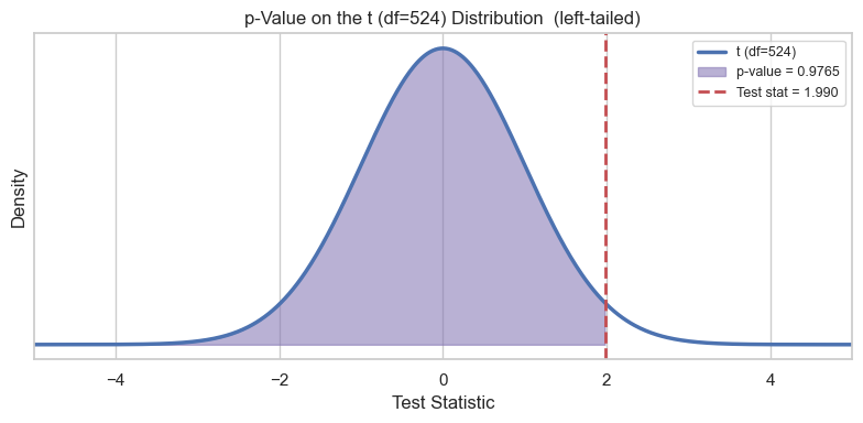

np.float64(0.9764691345103486)

# Step 5 — Make a decision
if p_value < alpha:
    print(f"p-value ({p_value:.4f}) < α ({alpha}) → Reject H₀")
    print("Conclusion: At the 5% significance level, there is sufficient evidence that")
    print(f"the mean NBA salary is greater than ${mu_0:,.0f}.")
else:
    print(f"p-value ({p_value:.4f}) ≥ α ({alpha}) → Fail to Reject H₀")
    print("Conclusion: At the 5% significance level, there is not sufficient evidence that")
    print(f"the mean NBA salary is greater than ${mu_0:,.0f}.")

p-value (0.0235) < α (0.05) → Reject H₀
Conclusion: At the 5% significance level, there is sufficient evidence that
the mean NBA salary is greater than $7,500,000.

5.3. Textbook-Style Check¶

OpenStax Chapter 9 emphasizes the manual test setup and decision rule. Below, we re-check our computed values using the same t-statistic and p-value formulas (no one-line test shortcut).

# Re-check with textbook formulas
t_check = (x_bar - mu_0) / se
p_check = stats.t.sf(t_check, df)

print(f"t statistic (check) = {t_check:.4f}")
print(f"p-value   (check)   = {p_check:.4g}")
print()
print(f"Matches Step 3 t-stat? {np.isclose(t_check, t_stat)}")
print(f"Matches Step 4 p-value? {np.isclose(p_check, p_value)}")

t statistic (check) = 1.9904
p-value   (check)   = 0.02353

Matches Step 3 t-stat? True
Matches Step 4 p-value? True

Question 5.1 (Code Practice — instructor solution). The next cell tests whether the mean NBA salary is different from $7.5M (two-tailed: H₀: μ = 7,500,000 vs Hₐ: μ ≠ 7,500,000).

We use $7.5M so (|t|) is moderate and the p-value shows up clearly in decimal form (compare to §5.2, which used the same threshold but a one-tailed test). The two-tailed p-value is 2 * stats.t.sf(abs(t), df) — double the upper-tail probability because extremes in either direction count against H₀.

# Instructor solution: two-tailed t-test vs μ₀ = $7.5M (uses x_bar, se, df from §5.2)
mu_0_new = 7_500_000

t_stat_new = (x_bar - mu_0_new) / se
p_value_new = 2 * stats.t.sf(abs(t_stat_new), df)  # two-tailed; same as 2 * (1 - cdf(|t|))

print(f"t statistic = {t_stat_new:.4f}")
print(f"p-value     = {p_value_new:.4f}")

if p_value_new < alpha:
    print("→ Reject H₀")
else:
    print("→ Fail to Reject H₀")

t statistic = 1.9904
p-value     = 0.0471
→ Reject H₀

Question 5.2 (Free Response). Based on your result above, write a one-sentence plain-English conclusion for the two-tailed test (H₀: μ = $7.5M). Make sure to mention the significance level and the direction of the evidence.

Your Answer Here

6. Test 2 — Population Proportion (z-Test)¶

6.1. When to Use a Proportion z-Test¶

Use a one-sample proportion z-test when:

You want to test a claim about a population proportion p (a fraction or percentage)
Each observation is a binary outcome — success or failure (e.g., “scores ≥ 15 points” or not)
The sample is large enough: both $np_0 ≥ 5$ and $n(1-p_0) ≥ 5$

The z-statistic formula for a proportion is:

z = \frac{\hat{p} - p_0}{\sqrt{p_0(1-p_0)/n}}

(10)

Where:

$\hat{p}$ = sample proportion (observed fraction of successes)
$p_0$ = claimed proportion from H₀
$n$ = sample size

The z-statistic uses the standard normal distribution (z-distribution).

6.2. NBA Example: Is More Than 15% of Players High Scorers?¶

We define a “high scorer” as any player averaging 15+ points per game.

Research question: Among all NBA players like those in this table, is the proportion of high scorers greater than 15%?

Step 1 — Hypotheses:
H₀: p ≤ 0.15 (at most 15% of players are high scorers)
Hₐ: p > 0.15 (more than 15% are high scorers) → right-tailed

Step 2 — Significance level: α = 0.05

Why test against 15% (not, say, 30%)? In this sample, about 17.7% score 15+ points, so $\hat p$ is above $p_0=0.15$ and the z-statistic for Hₐ: p > 0.15 is positive — the right-tail p-value is a small decimal you can read in the output and on the plot. If we instead tested Hₐ: p > 0.30, $\hat p$ would be below 0.30, z would be negative, and the correct right-tail p-value P(Z > z) would be close to 1 (often printing as 1.0000) even though that only means “no evidence above 30%.”

# Step 3 — Compute sample proportion
threshold = 15       # points per game to be a "high scorer"
p_0       = 0.15     # H0 boundary (see §6.2 — chosen so z and p-value are easy to read)

n_prop    = len(nba_clean["Points"].dropna())
successes = (nba_clean["Points"] >= threshold).sum()
p_hat     = successes / n_prop

print(f"Total players     n  = {n_prop}")
print(f"High scorers (≥15) x  = {successes}")
print(f"Sample proportion p̂  = {p_hat:.4f}  ({p_hat*100:.1f}%)")
print()
# Check assumptions
print(f"np₀ = {n_prop * p_0:.1f}  (need ≥ 5 ✓ if > 5)")
print(f"n(1-p₀) = {n_prop * (1 - p_0):.1f}  (need ≥ 5 ✓ if > 5)")

Total players     n  = 525
High scorers (≥15) x  = 93
Sample proportion p̂  = 0.1771  (17.7%)

np₀ = 78.8  (need ≥ 5 ✓ if > 5)
n(1-p₀) = 446.2  (need ≥ 5 ✓ if > 5)

# Step 3 continued — compute the z-statistic
se_prop = np.sqrt(p_0 * (1 - p_0) / n_prop)
z_stat  = (p_hat - p_0) / se_prop

print(f"Standard error = {se_prop:.6f}")
print(f"z statistic    = ({p_hat:.4f} - {p_0}) / {se_prop:.6f}")
print(f"z statistic    = {z_stat:.4f}")

Standard error = 0.015584
z statistic    = (0.1771 - 0.15) / 0.015584
z statistic    = 1.7417

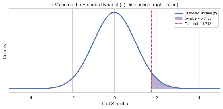
# Step 4 — p-value (right-tailed)
p_value_prop = stats.norm.sf(z_stat)   # P(Z > z_stat)

print(f"p-value = {p_value_prop:.4f}")  # with p₀ = 0.15 and p̂ ≈ 0.18, p is ~0.04 (not ~1)

# Visualize on the standard normal curve
_ = show_pvalue_visual(test_stat=z_stat, tail="right", distribution="z")

p-value = 0.0408

# Step 5 — Decision
pct = int(round(p_0 * 100))
if p_value_prop < alpha:
    print(f"p-value ({p_value_prop:.4f}) < α ({alpha}) → Reject H₀")
    print("Conclusion: At the 5% level, there is sufficient evidence that more than")
    print(f"{pct}% of NBA players average 15+ points per game.")
else:
    print(f"p-value ({p_value_prop:.4f}) ≥ α ({alpha}) → Fail to Reject H₀")
    print("Conclusion: At the 5% level, there is not sufficient evidence that more than")
    print(f"{pct}% of NBA players average 15+ points per game.")

p-value (0.0408) < α (0.05) → Reject H₀
Conclusion: At the 5% level, there is sufficient evidence that more than
15% of NBA players average 15+ points per game.

Question 6.1 (Code Practice — instructor solution). The next cell tests whether the proportion of players averaging 20+ points is different from 10% (two-tailed).

# Instructor solution: two-tailed proportion z-test (20+ points vs p₀ = 0.10)
threshold_new = 20
p_0_new       = 0.10

successes_new = (nba_clean["Points"] >= threshold_new).sum()
p_hat_new     = successes_new / n_prop
se_new        = np.sqrt(p_0_new * (1 - p_0_new) / n_prop)
z_stat_new    = (p_hat_new - p_0_new) / se_new
p_value_new   = 2 * (1 - stats.norm.cdf(abs(z_stat_new)))  # two-tailed

print(f"Sample proportion p̂ = {p_hat_new:.4f}")
print(f"z statistic          = {z_stat_new:.4f}")
print(f"p-value              = {p_value_new:.4f}")

if p_value_new < alpha:
    print("→ Reject H₀")
else:
    print("→ Fail to Reject H₀")

Sample proportion p̂ = 0.0895
z statistic          = -0.8001
p-value              = 0.4236
→ Fail to Reject H₀

Question 6.2 (Free Response). In your own words, explain the difference between the t-test (Section 5) and the proportion z-test (Section 6). When would you use each one? Give one example NBA question for each.

Your Answer Here

7. Sandbox: Your Own Hypothesis Test¶

Now it’s your turn! Use the interactive widgets below to run your own hypothesis tests on any column in the NBA dataset.

Pick a claim you find interesting — maybe about assists, rebounds, age, or minutes played — and test it!

7.1. One-Sample t-Test (Mean)¶

# Choose a column, a hypothesized mean, and a tail → click Run t-Test
show_ttest_sandbox(nba_clean)

7.2. One-Sample Proportion z-Test¶

# Choose a column, a success threshold, a claimed proportion, and a tail
show_proportion_sandbox(nba_clean)

Question 7.1 (Free Response). Choose one test you ran above (t-test or proportion test). Write up your findings using the five-step format:

H₀:
Hₐ:
Test statistic:
p-value:
Conclusion (in plain English at the 5% significance level):

Your Answer Here

Conclusion¶

In this notebook, we covered the core ideas of Hypothesis Testing with One Sample:

Every test starts by stating H₀ and Hₐ — only then do you touch the data.
The tail of the test (left / right / two) is determined entirely by Hₐ.
A Type I error (false alarm) happens when you reject a true H₀ — its probability is α.
A Type II error (miss) happens when you fail to reject a false H₀ — its probability is β.
The p-value measures how surprising your data is if H₀ were true. When p < α → Reject H₀.
Use a t-test to test a claim about a population mean (unknown σ).
Use a proportion z-test to test a claim about a population proportion.

These tools are the backbone of statistical inference. Great work! 🎉

📋 Post-Notebook Reflection Form¶

Thank you for completing the notebook! We’d love to hear your thoughts so we can continue improving.

👉 Click here to fill out the Reflection Form

🧠 Why it matters:¶

Your feedback helps us understand:

How clear and helpful the notebook was
What you learned from the experience
What topics you’d like to see in the future

This form is anonymous and takes less than 5 minutes. We appreciate your input! 💬

Woohoo! You have completed this notebook! 🚀

Hypothesis Testing with One Sample (Instructor — solutions filled in)

Table of Contents¶

Notebook Structure¶

1. Quick Concepts and Setup¶

1.1. Learning Objectives¶

1.2. The Big Picture¶

1.3. Setup¶

1.4. Load the Data¶

2. Null and Alternative Hypotheses¶

2.1. Setting Up Your Hypotheses¶

2.2. Left-, Right-, and Two-Tailed Tests¶

3. Type I and Type II Errors¶

3.1. The Error Table¶

3.2. Seeing the Trade-Off¶

4. The p-Value and Decision Rule¶

4.1. What is a p-Value?¶

4.2. Decision Rule¶

5. Test 1 — Population Mean (t-Test)¶

5.1. When to Use a t-Test¶

5.2. NBA Example: Is the Average Salary Greater Than $7.5M?¶

Quick Note: What do t.cdf and norm.cdf mean?¶

5.3. Textbook-Style Check¶

6. Test 2 — Population Proportion (z-Test)¶

6.1. When to Use a Proportion z-Test¶

6.2. NBA Example: Is More Than 15% of Players High Scorers?¶

7. Sandbox: Your Own Hypothesis Test¶

7.1. One-Sample t-Test (Mean)¶

7.2. One-Sample Proportion z-Test¶

Conclusion¶

📋 Post-Notebook Reflection Form¶

🧠 Why it matters:¶

Quick Note: What do `t.cdf` and `norm.cdf` mean?¶